
library(tidyverse)       # ggplot, dplyr, %>%, and friends
library(brms)            # bayesian models
library(catR)            # for IRT simulations
library(DT)              # for interactive tables
library(tidybayes)       # for extracting info from the brms model
library(patchwork)       # combine multiple ggplots
library(ggtext)          # for adding text to plots
library(gridtext)        # for adding text to plots
library(marginaleffects) # to calculate average value for demographic groups from model


# Custom ggplot theme to make pretty plots
# Get the News Cycle font at https://fonts.google.com/specimen/News+Cycle
theme_clean <- function() {
  theme_minimal(base_family = "News Cycle") +
    theme(panel.grid.minor = element_blank(),
          plot.title = element_text(face = "bold"),
          axis.title = element_text(face = "bold"),
          strip.text = element_text(face = "bold", size = rel(1), hjust = 0),
          strip.background = element_rect(fill = "grey80", color = NA),
          legend.title = element_text(face = "bold"))
}It has been nearly 7 years since I defended my PhD dissertation on language attitudes on Pohnpei in the Federated States of Micronesia and over 8 years since I collected data for it! I have learned a lot since that time and want to revisit one of the analyses from my dissertation to see if I can create a more robust version using Bayesian item response theory (IRT) models. In this blog post, we will explore using Bayesian IRT to model English language use on Pohnpei.
To get started we will be using these packages.
What is Item Response Theory?
IRT is a family of statistical models that aims to describe the relationship between a latent ability/value measured by an instrument (such as a test or questionnaire) and an individual’s response to each item on the instrument. IRT models generally provide us with these metrics about the topic being measured:
- A continuous ability score for each respondent. These values are often scaled so that they essentially represent z-scores, where the average value is 0 and the standard deviation is 1.
- A difficulty value1 for each item. Difficulty values are on the same scale as the ability scores and indicate the ability level needed to have a 50% probability of answering the item correctly (for tests) or endorsing a specific value (questionnaires).
- A discrimination value for each item that represents the item’s ability to distinguish between different ability levels. In some IRT models (such as 1-parameter models), the discrimination value is held constant across all items, and in others (such as 2-parameter models) it is allowed to vary for each item.
- More complicated IRT models allow additional metrics like guessing values (3-parameter models) and upper asymptote values (4-parameter models), but we won’t discuss those.
1 In some models you get an easiness value instead which is -1 * the difficulty value.
How does all of this differ from the old way (classical test theory), where we just sum together the number of correct responses and use that as a score? The old way assumes that all items have equal weight when creating the score. That means that if an individual answered 43/50 items correct and another individual also answered 43/50 items correct, but not the exact same 43 items, they would still have the same score. The sum score doesn’t tell us anything about the items themselves, just the percentage overall correct. We, therefore, have a hard time comparing values between respondents, since unless you get a perfect 50/50 or 0/50, we can’t directly compare values because they could mean different things.
IRT analyses solve this problem by assigning weights to each item by how difficult each item is and how well it distinguishes between ability levels. If a respondent correctly answers a harder item, then that means that they likely have a higher ability level than if they only correctly answered easier items. Therefore, each combination of responses corresponds to a unique ability score (at least with IRT models that use 2 or more parameters). Those ability scores are unambiguous and can be compared between individuals and even with the items. To see this in action, we’ll generate 50 items that each have a different difficulty value following a standard normal distribution. Then for each possible number of items correct (1–50 items),2 we randomly select that number of items 100 times and assume the respondent answered those items correctly and the rest incorrectly. We then calculate the latent ability value, \(\theta\), using thetaEst() for each iteration and plot them to show the possible variation. The graph shows that there can be a fair amount of ability variation even though respondents answered the same number of items correctly.
2 We skip 0 since the thetaEst() function breaks with 0 correct items.
# generate 50 items
fake_items <- tibble(item = 1:50,
                     difficulty = rnorm(50),
                     discrimination = runif(50,min = 0.3,max = 3))

# set the number of possible correct items
n_values <- seq(1, 50, by = 1)

# Create all combinations of n_values and iterations
sim_grid <- crossing(
  n_items = n_values,
  iteration = 1:100  # 100 iterations per n_value
)

# function to calculate thetas
estimate_theta <- function(n_items, iteration) {
  # Select items to mark as correct
  correct_items <- fake_items %>%
    slice_sample(n = n_items, replace = FALSE)

  # Create full response vector (1 = correct, 0 = incorrect)
  response_vector <- fake_items %>%
    mutate(resp = as.integer(item %in% correct_items$item)) %>%
    pull(resp)
  # create the irt parameters in right format for thetaEst
  item_params <- cbind(a = fake_items$discrimination,
                       b = fake_items$difficulty,
                       c = 0, #  guessing set to 0
                       d = 1) # upper asymptote set to 1

  thetaEst(item_params,
           response_vector,
           method = "EAP") %>%
    as_tibble() %>%
    mutate(
      n_items = n_items,
      iteration = iteration,
      n_correct = n_items
    ) %>%
    rename(theta = value)
}

# Run all combinations using pmap()
theta_results <- pmap(sim_grid, estimate_theta) %>%
  list_rbind()

# Plot results
theta_results %>%
  ggplot(aes(x = n_correct, y = theta)) +
  geom_point() +
  ylab("IRT Theta (Ability Score)") +
  xlab("Number of Items Correct") +
  theme_clean()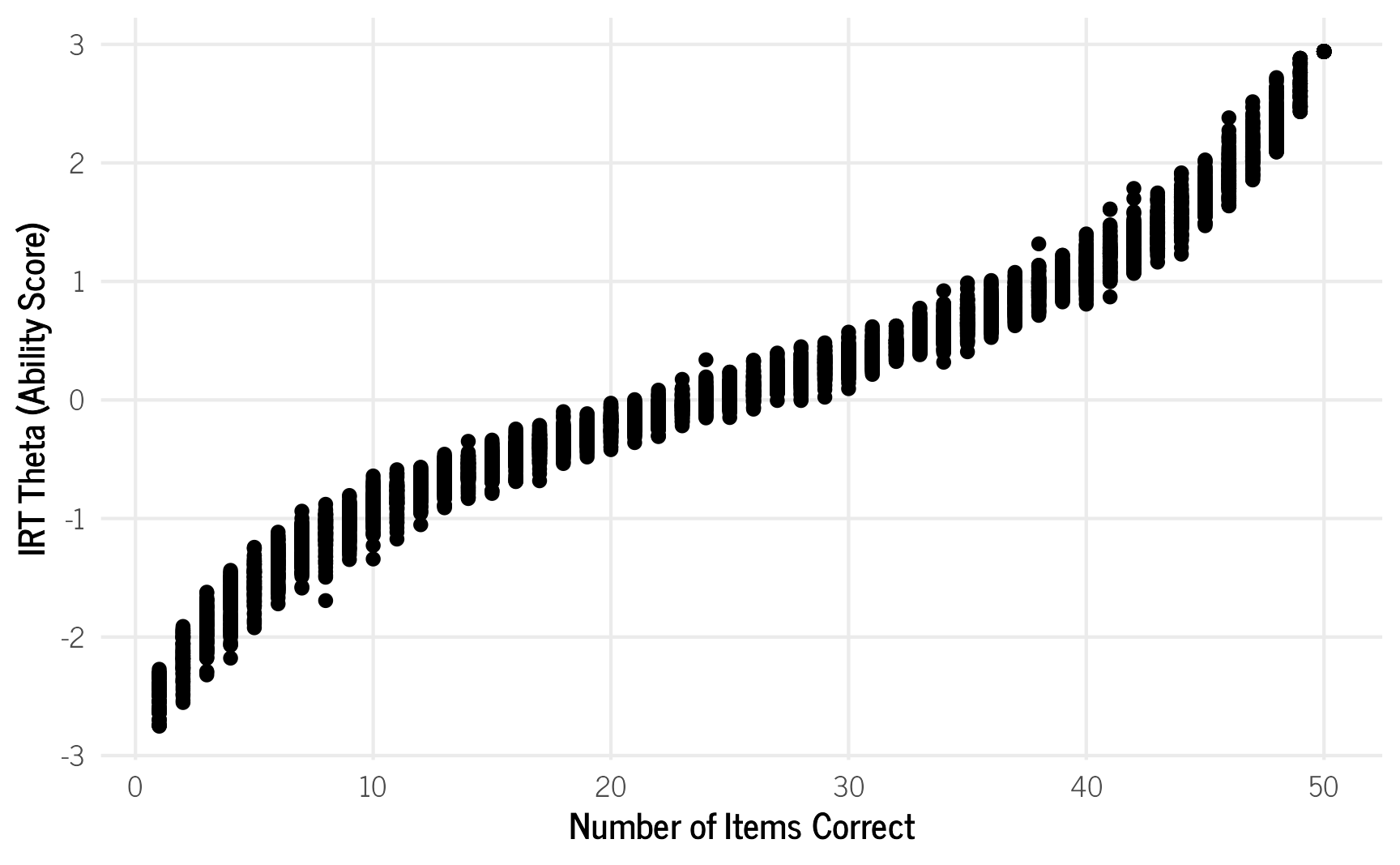
IRT models have two additional benefits. First, IRT models allow us to see how well our instrument measures ability level across the entire range of possible ability levels. That means that the researcher can assess if the instrument is biased toward specific ability levels and can thus add, remove, or modify items to get the desired measurement accuracy for the range of interest for the ability values. Second, IRT models are sample independent, so can be administered to different samples and the scores can be equated as needed. This is useful if we want to measure the latent ability at multiple time points or to different groups of the same population. In terms of measuring language attitudes and language use, these benefits are crucial, since we want to accurately measure the full range of language attitudes and use within a community, and we want to be able to track that use over time and possibly compare it to other communities.
Prepping the Data
For this analysis we will be using the data from a survey administered to 301 people on Pohnpei between June 2016 and August 2017. The original data and code can be found in the GitHub repo for my dissertation, but the file we are using needs to be created using multiple of the original files. For convenience the file we are using is located here.
We are interested in examining which domains of language use on Pohnpei are associated most with English and how that varies by different demographic groups. So we import the data and select only those variables. In the original survey, respondents were asked to select which language (among a choice of languages commonly spoken on Pohnpei) was most important to them in 25 different domains.3 Since we are focusing on English use, we recode those language choices to 1 if English and 0 if not. We also need the data in a long format, so we pivot all the domain items into two columns: domain and language.
3 Throughout this post I use English use and English importance fairly interchangeably, but they are technically different things, since importance doesn’t always translate to actual use. And of course a questionnaire only captures a snapshot of a respondent’s views. I chose English use as a more intuitive term for the sake of this post. See my dissertation for a more nuanced description of what the questionnaire items mean and how they were created.
The demographic variables that we have available in the data are the respondent’s age, gender, their current municipality of residence on Pohnpei, highest educational attainment, the type of elementary school they attended (public, private, or both types), and type of high school attended (none, public, private, or both types). For this blog post, we’ll skip some of the demographic variables I used in my dissertation like place of birth and whether they have traveled abroad.
data <- read_rds("data/complete_survey_data.rds")

# select demographic variable
demos <- data %>%
  select(questionnaire_id,
         age,sex,
         current_muni,
         education,
         elementary_type,
         hs_type, current_village) %>%
  # recode age due to small n for 75+
  mutate(age = case_when(
    age == "65 -- 74" ~ "65+",
    age == "75+" ~ "65+",
    .default = age
  )) %>%
  # recode current municipality to split Kolonia from Nett
  mutate(current_muni = case_when(
    current_village %in% c("Kolonia","Chinatown","Dolonier","Mabusi","Pohnrakied") ~ "Kolonia",
    .default = current_muni
  )) %>%
  dplyr::select(-current_village) %>%
  drop_na()

# select domains
domains <- data %>% dplyr::select(questionnaire_id,
                                  making_friends:us_relatives) %>%
  pivot_longer(making_friends:us_relatives,
               names_to="domain",
               values_to = "language") %>%
  mutate(english = case_when(
    language == "English" ~ 1,
    is.na(language) == TRUE ~ NA, # keep NAs as NA
    .default = 0
  ))

# combine back together
irt_data <- domains %>%
  inner_join(demos) %>%
  # convert demographics to factor
  mutate(across(age:hs_type, ~ as.factor(.))) %>%
  rename(gender = sex)

irt_data %>%
  head() %>%
  datatable()
Creating the IRT Model
Unlike with frequentist IRT models, we don’t have an off-the-shelf function that runs the model for us. Instead we have to more manually specify the formula for the model, like we would with a regular regression model. To do this, I will adjust code for the 2-parameter IRT model from Paul-Christian Bürkner’s article about creating IRT models with the brms package and A. Solomon Kurz’s post on making ICC plots for brms IRT models.
Let’s call our binary outcome of selecting English in a given domain, \(y_{pd}\), which varies across \(P\) persons and \(D\) domains. This follows a Bernoulli distribution, where \(p_{pd}\) is the probability of selecting English for the p-th person on the d-th domain. The logit link sets the probabilities to [0, 1] for us. The probability of selecting English is equal to the item’s discrimination, \(\alpha\), times the sum of the grand mean, \(\beta_0\), the respondent’s latent ability, \(\theta_p\), the domain’s easiness4 value, \(\xi_d\), as well as variation due to the vector of demographic variables, \(\mathbf{\Gamma}_p \cdot \beta_\Gamma\). In order to make sure the model’s results are interpretable, we log the discrimination value to ensure it is positive. We put this all together in math notation like this:5
4 Because of model specification issues, this value represents the easiness of selecting English in that domain, which is just -1*difficulty. We’ll switch it back to difficulty later.
5 I did not include \(\alpha\) and \(\xi\) covariance and correlation matrices in the equation, but are included in the model. See the two sources cited at the beginning of this section for additional details.
\[\begin{split}y_{pd} &\sim \operatorname{Bernoulli}(p_{pd}) \\ \operatorname{logit}(p_{pd}) &= \operatorname{exp(log} \alpha) \times (\beta_0 + \theta_p + \xi_d + \mathbf{\Gamma}_p \cdot \beta_\Gamma) \\ \operatorname{log} \alpha &= \beta_1 + \alpha_d \\ \theta_p &\sim \operatorname{Normal}(0,\sigma_\theta)\end{split} \] To simplify things further, we can rewrite \((\beta_0 + \theta_p + \xi_d + \mathbf{\Gamma}_p \cdot \beta_\Gamma)\) as \(\eta\) and model it as a latent variable:
\[\begin{split}y_{pd} &\sim \operatorname{Bernoulli}(p_{pd}) \\ \operatorname{logit}(p_{pd}) &= \operatorname{exp(log} \alpha) \times \eta \\ \eta &= \beta_0 + \theta_p + \xi_d + \mathbf{\Gamma}_p \cdot \beta_\Gamma \\ \operatorname{log} \alpha &= \beta_1 + \alpha_d \\ \theta_p &\sim \operatorname{Normal}(0,\sigma_\theta)\end{split} \] Because we are modeling latent variables, we can use our priors to help ensure interpretability of the values. We set the standard deviation of the person parameter as a constant of 1, \(\sigma_\theta=1\), so that the person parameters are essentially z-scores, and use the weakly informative priors for the betas and the other sigmas of \(\operatorname{Normal}(0,1)\).
These are the priors we set: \[\begin{split} \beta_0 &\sim \operatorname{Normal}(0,1)\\ \beta_1 &\sim \operatorname{Normal}(0,1)\\ \beta_\Gamma &\sim \operatorname{Normal}(0,1)\\\sigma_\theta&=1\\ \sigma_\alpha &\sim\operatorname{Normal}(0,1)\\\sigma_\xi&\sim \operatorname{Normal}(0,1)\\ \mathbf{R} &\sim \operatorname{LKJ}(2) \end{split}\] The last prior we set to weakly regularize the correlation matrix, \(\mathbf{R}\).
Let’s convert this all to brms code and run the model.
# set contrasts for demos so that intercept is grand mean
contrasts(irt_data$age) <- contr.sum
contrasts(irt_data$education) <- contr.sum
contrasts(irt_data$current_muni) <- contr.sum
contrasts(irt_data$elementary_type) <- contr.sum
contrasts(irt_data$hs_type) <- contr.sum
contrasts(irt_data$gender) <- contr.sum

# set the formula
formula_2pl <- bf(
  english ~ exp(logalpha) * eta,
  eta ~ 1 + age + gender + current_muni + education + elementary_type * hs_type +
    (1 |i| domain) + # |i| models the domain correlation between eta and alpha
    (1 | questionnaire_id), # this is the ID by person
  logalpha ~ 1 + (1 |i| domain), # model discrimination by each domain (aka item)
  nl = TRUE # need to set non-linear to True since we have latent variables
)

# set priors
priors_2pl <-
  prior(normal(0,1), class = "b", nlpar = "eta") + # prior betas for eta
  # priors for domains (aka items) for easiness and discrimination
  prior(normal(0,1), class = "sd", group = "domain", nlpar = "eta") +
  prior(normal(0,1), class = "sd", group = "domain", nlpar = "logalpha") +
  # constrain the variance for person parameters to 1 so that the results are identifiable
  prior(constant(1), class = "sd", group = "questionnaire_id", nlpar = "eta") +
  # prior for discrimination intercept
  prior(normal(0.5,1), class = "b", nlpar = "logalpha") +
  # prior to regularize item parameter correlations
  prior(lkj(2), class = "cor", group = "domain")

domains_eng_irt <- brm(formula = formula_2pl,
                       data = irt_data,
                       prior = priors_2pl,
                       family = bernoulli(),
                       iter = 2000,
                       chains = 4,
                       cores = 4)
Results
How well did the model measure English use?
We can calculate how much information the questionnaire provides across values of the latent English language use variable as a way to measure how well the questionnaire performed. Information for a given value of the latent variable, \(\theta\) is calculated by
\[ I(\theta) = \alpha^2_d p_d(\theta) q_d(\theta)\] where \(\alpha_d\) is the discrimination value for each domain, \(p_d(\theta)\) is the probability of selecting English for a given ability level \(\theta\) and \(q_d(\theta)\) is the probability of not selecting English, which is \(1-p_d(\theta)\). We calculate the information provided by the questionnaire for \(\theta\) values -6–6.
# Extract draws and compute information
info_data <- as_draws_df(domains_eng_irt) %>%
  # Select relevant parameters
  dplyr::select(.draw, b_eta_Intercept, b_logalpha_Intercept,
                starts_with("r_domain")) %>%
  # Reshape to long format
  pivot_longer(starts_with("r_domain")) %>%
  # Extract item and parameter type
  mutate(
    item = str_extract(name, "(?<=\\[).*?(?=,)"),
    parameter = case_when(
      str_detect(name, "eta") ~ "eta_r",
      str_detect(name, "logalpha") ~ "logalpha_r"
    )
  ) %>%
  dplyr::select(-name) %>%
  # Separate into different columns
  pivot_wider(names_from = parameter, values_from = value) %>%
  # Compute IRT parameters
  mutate(
    a_i = exp(b_logalpha_Intercept + logalpha_r),  # Discrimination parameter
    b_i = -(b_eta_Intercept + eta_r)               # Difficulty parameter
  ) %>%
  # Create theta grid
  expand(nesting(.draw, item, a_i, b_i),
         theta = seq(-6, 6, length.out = 200)) %>%
  # Compute probabilities and information
  mutate(
    p = plogis(a_i * (theta - b_i)),
    info = a_i^2 * p * (1 - p)
  )

# Compute test information by summing across items
test_info_summary <- info_data %>%
  # Sum information across items within each draw/theta combination
  group_by(.draw, theta) %>%
  summarise(test_info = sum(info), .groups = "drop") %>%
  # Summarize across draws
  group_by(theta) %>%
  median_qi(test_info)  # Median and 95% quantile intervals

# Plot the TIC with uncertainty
ggplot(test_info_summary, aes(x = theta, y = test_info)) +
  geom_ribbon(aes(ymin = .lower, ymax = .upper),
              alpha = 0.3, fill = "#440154") +
  geom_line(linewidth = 1, color = "#440154") +
  labs(title = "Test Information Curve (TIC)",
       x = expression(theta~("English Use")),
       y = "Total Test Information",
       caption = "Ribbon shows 95% credible interval") +
  theme_clean() +
  theme(legend.position = "none")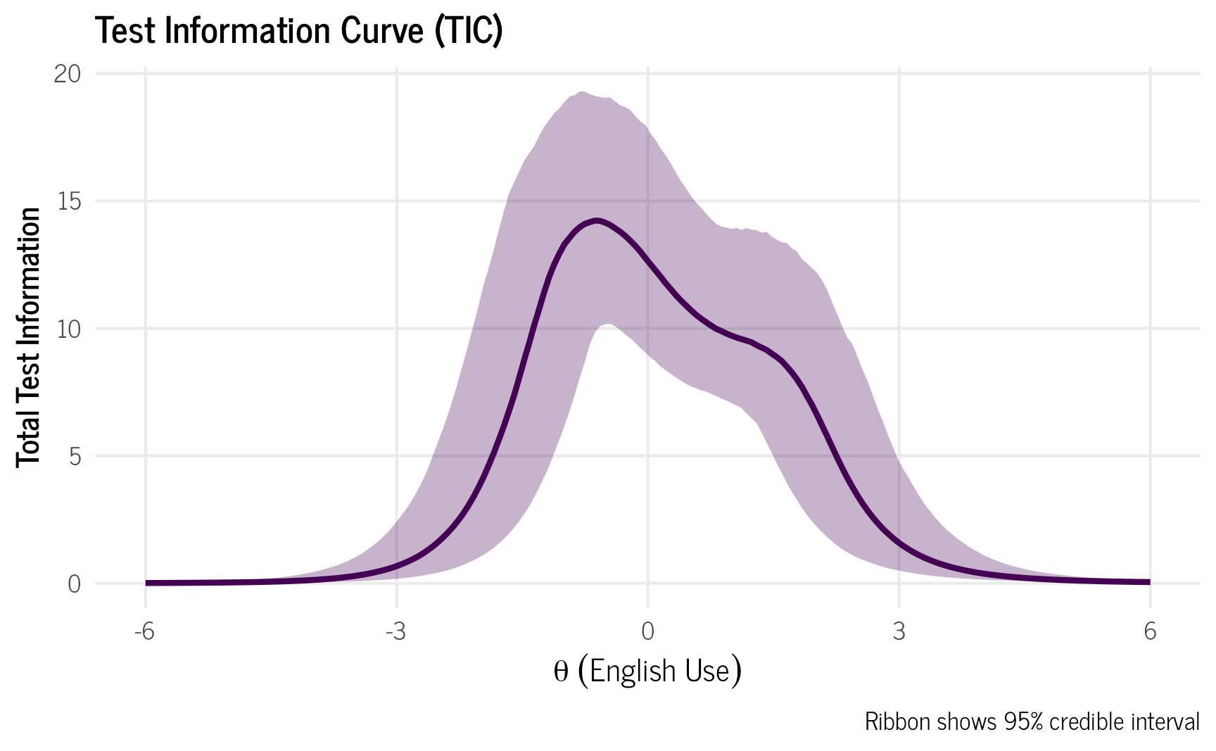
We can also convert the information values to standard error: \[ \operatorname{SE}(\theta) = \frac{1}{\sqrt{I(\theta)}}\]
# Compute test information by summing across items
test_info_summary <- info_data %>%
  # Sum information across items within each draw/theta combination
  group_by(.draw, theta) %>%
  summarise(test_info = sum(info), .groups = "drop") %>%
  mutate(test_se = 1 / sqrt(test_info)) %>%
  # Summarize across draws
  group_by(theta) %>%
  median_qi(test_se)  # Median and 95% quantile intervals

# Plot SE
ggplot(test_info_summary, aes(x = theta, y = test_se)) +
  geom_ribbon(aes(ymin = .lower, ymax = .upper),
              alpha = 0.3, fill = "#440154") +
  geom_line(linewidth = 1, color = "#440154") +
  labs(title = "Test Measurement Error Curve",
       x = expression(theta~("English Use")),
       y = "Standard Error",
       caption = "Ribbon shows 95% credible interval") +
  theme_clean() +
  theme(legend.position = "none")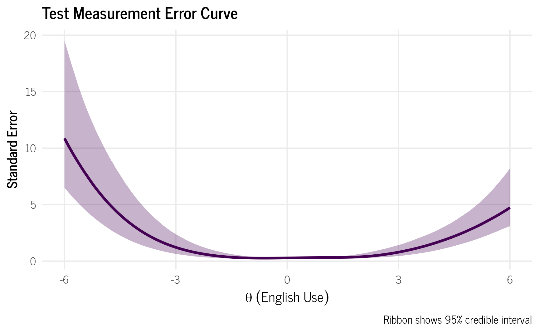
We can see from the two graphs, that the items provide the most information between English use values of -3 and 3. Since the English use values are essentially z-scores, \(\pm\) 3 would cover 99.7% of the population, which is enough for our purposes. If we were to do a classical test theory approach, we would only be able to calculate the reliability of the instrument on average, so we would not be able to know how the instrument performs at different values of \(\theta\).
How likely was it to select English for each domain?
We can extract the domain difficulties and discrimination values from the model to see how likely it was to select English for each domain.
# create function to extract IRT item parameters from model
extract_irt_items <- function(model, cri = 0.5){
  # extract item parameters
  lower_prob = (1 - cri)/2
  upper_prob = 1 - lower_prob
  item_coefs <- coef(model, probs = c(lower_prob,upper_prob))$domain
  # get etas for items (item easiness)
  eta <- item_coefs[, , "eta_Intercept"] %>%
    data.frame() %>%
    rownames_to_column()
  # get alphas for items (item discrimination)
  alpha <- item_coefs[, , "logalpha_Intercept"] %>%
    exp() %>%
    data.frame() %>%
    rownames_to_column()

  final_df <- bind_rows(eta, alpha, .id = "nlpar") %>%
    rename(item = "rowname") %>%
    mutate(nlpar = factor(nlpar,
                          labels = c("Easiness",
                                     "Discrimination"))) %>%
    rename(Parameter = nlpar)
  return(final_df)

}


domain_difficulty <- extract_irt_items(domains_eng_irt, cri = 0.50) %>%
  mutate(type = "Domain") %>%
  mutate(item = fct_recode(item,
                             "Being accepted in Pohnpei" = "accepted_pni",
                             "Being successful" = "being_successful",
                             "Going to church" = "church",
                             "Using Facebook" = "facebook",
                             "Talking with friends from school" = "friends_school",
                             "Attending funerals" = "funerals",
                             "Getting money" = "getting_money",
                             "Getting a good education" = "good_education",
                             "Getting a good job" = "good_job",
                             "Feeling happy in your relationships" = "happy_relationships",
                             "Attending a Kamadipw" = "kamadipw",
                             "Making friends" = "making_friends",
                             "Listening to the radio" = "radio",
                             "Reading" = "reading",
                             "Drinking Sakau en Pohnpei" = "sakau",
                             "Going to the store" = "store",
                             "Talking with a Kaunen Kousapw" = "talking_chief",
                             "Talking with government officials" = "talking_gov",
                             "Talking with people in Kolonia" = "talking_kolonia",
                             "Talking with your neighbors" = "talking_neighbors",
                             "Talking with teachers" = "talking_teachers",
                             "Talking with people in the villages of Pohnpei" = "talking_villages",
                             "Watching TV" = "tv",
                             "Speaking with relatives who live in the U.S." = "us_relatives",
                             "Writing" = "writing"
  ))

  diff_plot <- domain_difficulty %>%
    filter(Parameter == "Easiness") %>%
  mutate(across(Estimate:Q75, ~ .x *-1)) %>%  # convert easiness to difficulty
    ggplot(aes(reorder(item, Estimate),
             Estimate,
             ymin = Q25,
             ymax = Q75)) +
  geom_pointrange() +
  coord_flip() +
  labs(x = "", y = "English Use Difficulty",
      ) +
  theme_clean() +
  theme(panel.grid.major.y = element_blank())

  discrim_plot <- domain_difficulty %>%
    filter(Parameter == "Discrimination") %>% ggplot(aes(reorder(item, Estimate),
             Estimate,
             ymin = Q25,
             ymax = Q75)) +
  #facet_wrap("Parameter", scales = "free_x") +
  geom_pointrange() +
  coord_flip() +
  labs(x = "", y = "Discrimation",
      ) +
  theme_clean() +
  theme(panel.grid.major.y = element_blank())

  diff_plot + discrim_plot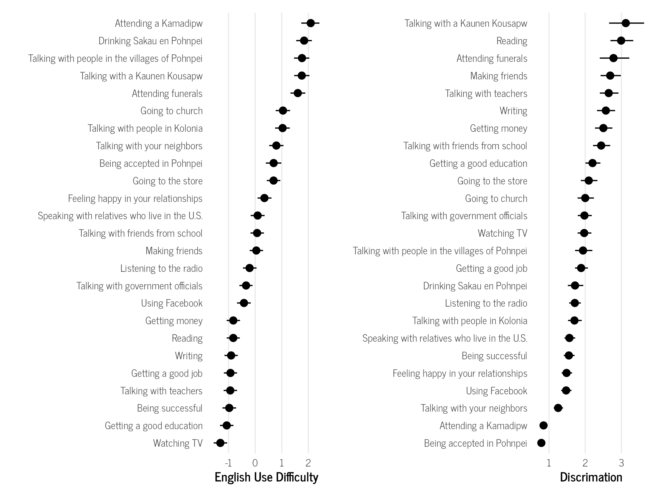
The English use difficulty values represent the latent ability needed in order to have a 50% probability of selecting English for each domain. Since the ability values are z-scores, 0 represents the average value, positive values have higher than average English use scores, and negative values have less than average English use scores. If an individual has the average English use score of 0, then they are likely to select English in all domains that have a difficulty value of 0 or less. This is a benefit of IRT analyses, where we can now say that if a person selects English for making friends, they will also likely select English for “easier” domains like reading and talking with teachers, but not in harder domains like when going to the store or when drinking Sakau. With classical test theory results, like the ones I used in my dissertation, we would not be able to make these inferences.
The discrimination values indicate how well the domain is at distinguishing different levels of English use abilities. Higher values indicate that the item is better at distinguishing than items with lower values. All but two items have discrimination values larger than 1, which is great! A rule of thumb that I learned at some point is that discrimination values should be larger than 0.65 to have “acceptable” discrimination. I have not seen any research to back that up. It could exist somewhere, or it could just be another one of those arbitrary rules that people are taught but are actually useless, wrong, outdated, or taken out of context.
Since the difficulty values are essentially z-scores, we can convert them to percentiles to see how likely the different English language use scores would be across the population.6 To do this, we use the easiness scores outputted from the model, instead of converting them to difficulty values, since as the name suggests, they represent how easy it is to use English in those domains. We see that only 1.9% of the population would be expected to select English as the most important language for attending a Kamadipw (a type of formal feast on Pohnpei), while 91% would select English for watching TV. Interestingly, 36% of the population would be expected to select English as the most important language for feeling happy in one’s relationships, and almost 50% would select English as the most important language for making friends. Now that we have the expected percentages, they could be tracked over time to measure how English language use changes over time, if the questionnaire were to be administered again.
6 This assumes the initial sample was representative of the population on Pohnpei.
domain_percentiles <- domain_difficulty %>%
    filter(Parameter == "Easiness") %>%
  mutate(across(Estimate:Q75, ~ pnorm(.x)))  # convert to percentile

domain_percentiles %>% ggplot(aes(reorder(item, Estimate),
             Estimate,
             ymin = Q25,
             ymax = Q75)) +
  geom_pointrange() +
  coord_flip() +
  labs(x = "", y = "Percentage Expected to Use English",
      ) +
  scale_y_continuous(labels = scales::percent) +
  theme_clean() +
  theme(panel.grid.major.y = element_blank())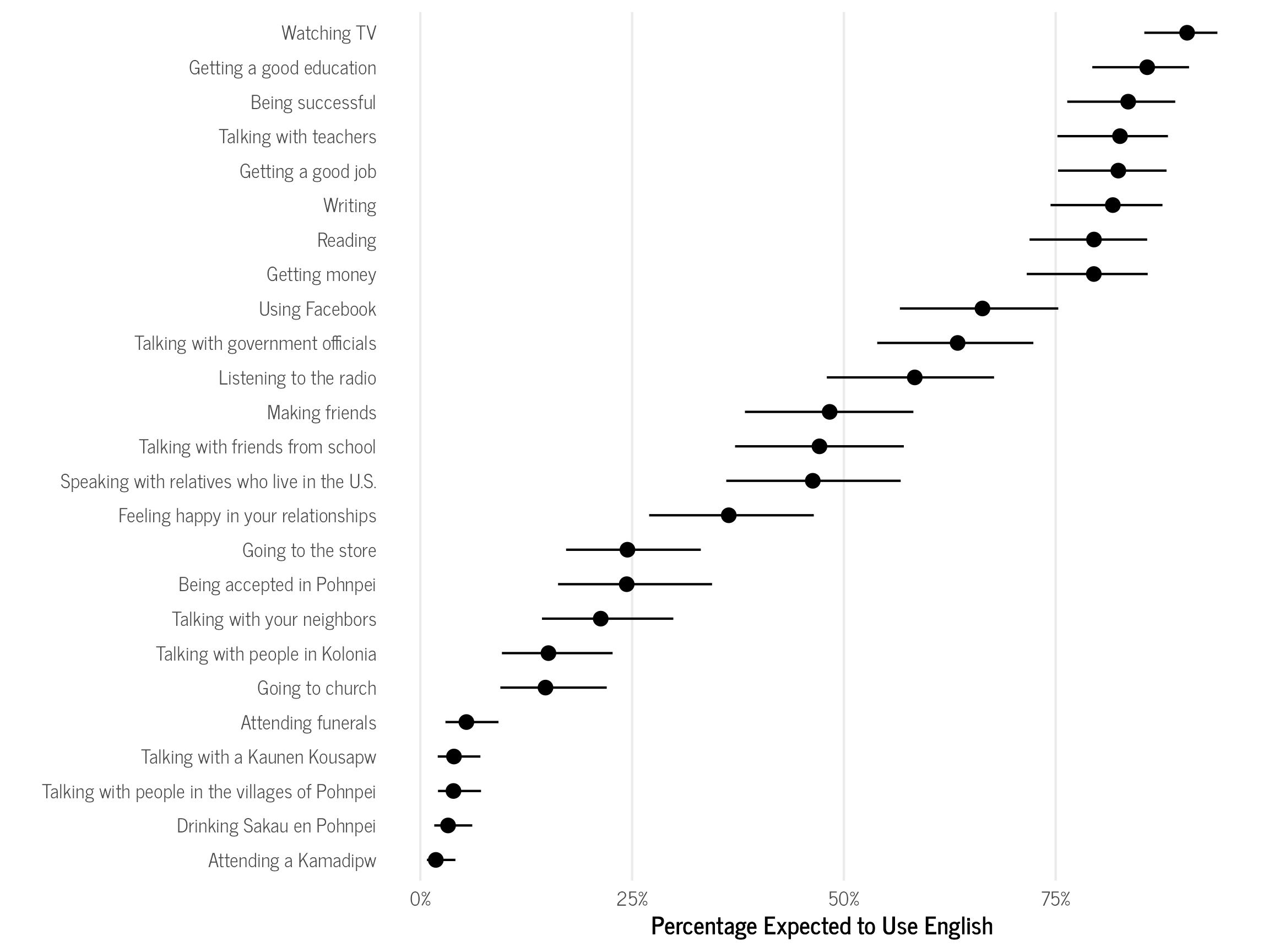
  domain_percentiles %>%
    arrange(-Estimate) %>%
    mutate(across(Estimate:Q75, ~ scales::percent(.x, accuracy = 0.1))) %>%
    dplyr::select(-type,-Parameter,-Est.Error) %>%
    datatable()
How does English language use vary by each demographic group?
One way to see how demographic groups vary in English language use is to calculate average predicted values using avg_predictions() in the marginaleffects package. We calculate the average predicted values for each demographic variable and then combine them with the previous values for domains that we calculated above so that we can directly compare each demographic group to the domains. In the graph below, each demographic group is likely to select English in each domain that has an equal or lesser value (all domains that occur to the left), but not those domains that have higher values (to the right).
# calculate average English score by group
elem <- avg_predictions(domains_eng_irt,
                by = "elementary_type",
                nlpar = "eta", # need to select the latent variable eta
                conf_level = 0.50,
                re_formula = NA) %>%
  data.frame() %>%
  rename(Estimate = estimate,
         Q25 = conf.low,
         Q75 = conf.high,
         item = elementary_type
         ) %>%
  mutate(Parameter = "Easiness",
         type = "Elementary Type",
         across(Estimate:Q75, ~ .x * -1)) # need to flip the sign to put on right scale

age <- avg_predictions(domains_eng_irt,
                        by = "age",
                        nlpar = "eta",
                        conf_level = 0.50,
                        re_formula = NA) %>%
  data.frame() %>%
  rename(Estimate = estimate,
         Q25 = conf.low,
         Q75 = conf.high,
         item = age
  ) %>%
  mutate(Parameter = "Easiness",
         type = "Age",
         across(Estimate:Q75, ~ .x * -1))

gender <- avg_predictions(domains_eng_irt,
                        by = "gender",
                        nlpar = "eta",
                        conf_level = 0.50,
                        re_formula = NA) %>%
  data.frame() %>%
  rename(Estimate = estimate,
         Q25 = conf.low,
         Q75 = conf.high,
         item = gender
  ) %>%
  mutate(Parameter = "Easiness",
         type = "Gender",
         across(Estimate:Q75, ~ .x * -1))

hs <- avg_predictions(domains_eng_irt,
                        by = "hs_type",
                        nlpar = "eta",
                        conf_level = 0.50,
                        re_formula = NA) %>%
  data.frame() %>%
  rename(Estimate = estimate,
         Q25 = conf.low,
         Q75 = conf.high,
         item = hs_type
  ) %>%
  mutate(Parameter = "Easiness",
         type = "HS Type",
         across(Estimate:Q75, ~ .x * -1))

education <- avg_predictions(domains_eng_irt,
                        by = "education",
                        nlpar = "eta",
                        conf_level = 0.50,
                        re_formula = NA) %>%
  data.frame() %>%
  rename(Estimate = estimate,
         Q25 = conf.low,
         Q75 = conf.high,
         item = education
  ) %>%
  mutate(Parameter = "Easiness",
         type = "Education Level",
         across(Estimate:Q75, ~ .x * -1))

current_muni <- avg_predictions(domains_eng_irt,
                        by = "current_muni",
                        nlpar = "eta",
                        conf_level = 0.50,
                        re_formula = NA) %>%
  data.frame() %>%
  rename(Estimate = estimate,
         Q25 = conf.low,
         Q75 = conf.high,
         item = current_muni
  ) %>%
  mutate(Parameter = "Easiness",
         type = "Current Municipality",
         across(Estimate:Q75, ~ .x * -1))

## combine with item parameters
domain_difficulty %>%
  filter(Parameter == "Easiness") %>%
  bind_rows(elem) %>%
  bind_rows(hs) %>%
  bind_rows(gender) %>%
  bind_rows(age) %>%
  bind_rows(education) %>%
  bind_rows(current_muni) %>%
  mutate(across(Estimate:Q75, ~ .x *-1)) %>%
  mutate(item.label = case_when(
    type == "Domain" ~ paste("<span style='color:gray50'>",
                         item,
                         "</span>", sep = ""),
    type == "Age" ~ paste("<span style='color:#66c2a5'>",
                          item,
                          "</span>", sep = ""),
    type == "Education Level" ~ paste("<span style='color:#fc8d62'>",
                                     item,
                                     "</span>", sep = ""),
    type == "Elementary Type" ~ paste("<span style='color:#8da0cb'>",
                                     item,
                                     "</span>", sep = ""),
    type == "Gender" ~ paste("<span style='color:#e78ac3'>",
                                     item,
                                     "</span>", sep = ""),
    type == "HS Type" ~ paste("<span style='color:#a6d854'>",
                                     item,
                                     "</span>", sep = ""),
    type == "Current Municipality" ~ paste("<span style='color:#e5c494'>",
                                     item,
                                     "</span>", sep = ""))) %>%
  ggplot(aes(reorder(item.label, Estimate),
             Estimate,
             ymin = Q25,
             ymax = Q75,
             color = type)) +
  geom_pointrange() +
  coord_flip() +
  labs(x = "", y = "English Use") +
  theme_clean() +
  scale_color_manual(values = c("#66c2a5",
                                "#e5c494",
                                "gray40",
                                "#fc8d62",
                                "#8da0cb",
                                "#e78ac3",
                                "#a6d854"
                                ),
                     name ="") +
  theme(axis.text.y = element_markdown(), panel.grid.major.y = element_blank())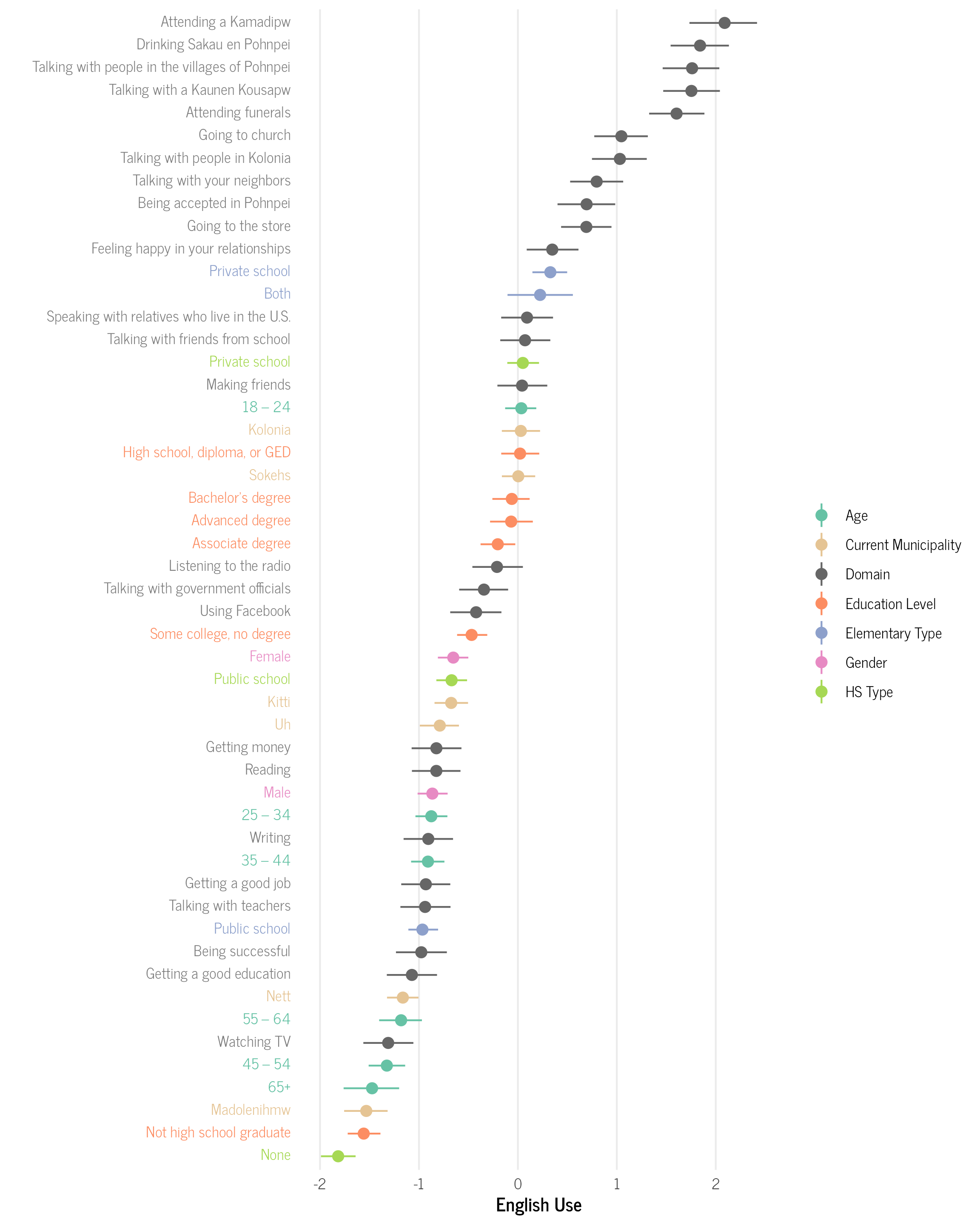
We see several interesting patterns among the demographics groups.
There are three general patterns for age groups. Those who were 45 or older tended to select English infrequently on average, such as for watching TV, getting a good education, being successful, and getting a good job. Those who were 25–44 selected English slightly more often than the older group, adding reading and getting money, but had similar patterns to the older group. The youngest group 18–24 selected substantially more English on average including feeling happy in your relationships, talking with friends from school, speaking with relatives who live in the U.S., making friends, listening to the radio, talking with government officials, and using Facebook. The oldest groups generally selected English for things that were heavily Western introduced like jobs, media, and American-style education, while the youngest group also selected English for more personal relationships like friends and some relatives. This pattern suggests a possible generational shift in language use.
There is fairly wide variation among the municipalities of Pohnpei. Madolenihmw, the most rural municipality, selected the least amount of English on average, similar to the oldest age group. Nett (excluding Kolonia) selected slightly more English than Madolenihmw, but still only for Western-introduced domains. Kitti and Uh have similar English use scores and are slightly higher than Nett. They have similar English use scores to the 25–44 age group. Finally, Kolonia and Sokehs, the two most urban and linguistically diverse municipalities, have similar English use scores to each other, but have substantially higher English use scores than the other municipalities, on par with the 18–24 age group. The more rural municipalities mostly selected English for Western-introduced domains, while the more urban municipalities also selected it for personal relationships.
For educational attainment, there are two general patterns. Those who did not graduate from high school selected very little English and patterned similarly to the oldest age group described above. Those who had completed high school, regardless of further educational attainment, patterned very similar to those who were aged 18–24. Completing western formal education correlates with substantial increased English use, including using English for personal relationships, like making friends.
Zooming in to the type of elementary school attended, those who attend only a public elementary school selected English primarily for Western-introduced domains, similar to the 25–44 age group. Those who attended a private elementary school or both a private and public one, had the highest English use values of any demographic group and selected English for more everyday interactions, including feeling happy in one’s relationship, being accepted in Pohnpei, and talking with your neighbors. This pattern is not surprising, since public elementary schools on Pohnpei have used local languages as a language of instruction for the early grades since the 1970s, while private elementary schools are English-only schools at all grade levels (some even punish students for using a language other than English). Elementary education is an important time for the development of one’s language skills and language attitudes.
When looking at the type of high school attended, there are similar patterns to the type of elementary school attended. Those who did not attend high school at all had the lowest English use scores of any group. They likely do not use English for any domain. Those who attended a public high school had somewhat higher English use scores than those who attended a public elementary. Those who attended a private high school had slightly lower English use scores than those who attended private elementary schools. While the effect of high school type follows a similar trend to type of elementary school attended, it is potentially noteworthy that the effect was smaller in magnitude, which suggests that the type of elementary school attended may have a stronger effect on one’s language use choices and attitudes.
Finally for gender, women had slightly higher English use scores than men. Men on average had values similar to those aged 25–44, and women had similar scores to those who attended a public high school.
We can also group the domains together into larger categories to see higher-level trends.
as_draws_df(domains_eng_irt) %>%
  # Select relevant parameters
  dplyr::select(.draw, b_eta_Intercept, b_logalpha_Intercept,
                starts_with("r_domain")) %>%
  # Reshape to long format
  pivot_longer(starts_with("r_domain")) %>%
  # Extract item and parameter type
  mutate(
    domain = str_extract(name, "(?<=\\[).*?(?=,)"),
    parameter = case_when(
      str_detect(name, "eta") ~ "eta_r",
      str_detect(name, "logalpha") ~ "logalpha_r"
    )) %>%
  dplyr::select(-name) %>%
  # Separate into different columns
  pivot_wider(names_from = parameter, values_from = value) %>%
  # Compute IRT parameters
  mutate(
    a_i = exp(b_logalpha_Intercept + logalpha_r),  # Discrimination parameter
    b_i = (b_eta_Intercept + eta_r)               # Easiness parameter
  ) %>%
  mutate(item = fct_recode(domain,
                           "Social Solidarity" = "accepted_pni",
                           "Occupation" = "being_successful",
                           "Pohnpei Customary Practice" = "church",
                           "Media" = "facebook",
                           "Education" = "friends_school",
                           "Pohnpei Customary Practice" = "funerals",
                           "Occupation" = "getting_money",
                           "Education" = "good_education",
                           "Occupation" = "good_job",
                           "Social Solidarity" = "happy_relationships",
                           "Pohnpei Customary Practice" = "kamadipw",
                           "Social Solidarity" = "making_friends",
                           "Media" = "radio",
                           "Media" = "reading",
                           "Pohnpei Customary Practice" = "sakau",
                           "General" = "store",
                           "Pohnpei Customary Practice" = "talking_chief",
                           "General" = "talking_gov",
                           "Social Solidarity" = "talking_kolonia",
                           "Social Solidarity" = "talking_neighbors",
                           "Education" = "talking_teachers",
                           "Social Solidarity" = "talking_villages",
                           "Media" = "tv",
                           "Social Solidarity" = "us_relatives",
                           "Education" = "writing"
  )) %>%
  group_by(item) %>%
  median_hdci(b_i,.width = 0.5) %>%
  rename(Estimate = b_i,
         Q25 = .lower,
         Q75 = .upper) %>%
  mutate(type = "Domain Group") %>%
  dplyr::select(-.width:-.interval) %>%
  bind_rows(elem) %>%
  bind_rows(hs) %>%
  bind_rows(gender) %>%
  bind_rows(age) %>%
  bind_rows(education) %>%
  bind_rows(current_muni) %>%
  mutate(across(Estimate:Q75, ~ .x *-1)) %>%
  mutate(item.label = case_when(
    type == "Domain Group" ~ paste("<span style='color:gray50'>",
                         item,
                         "</span>", sep = ""),
    type == "Age" ~ paste("<span style='color:#66c2a5'>",
                          item,
                          "</span>", sep = ""),
    type == "Education Level" ~ paste("<span style='color:#fc8d62'>",
                                     item,
                                     "</span>", sep = ""),
    type == "Elementary Type" ~ paste("<span style='color:#8da0cb'>",
                                     item,
                                     "</span>", sep = ""),
    type == "Gender" ~ paste("<span style='color:#e78ac3'>",
                                     item,
                                     "</span>", sep = ""),
    type == "HS Type" ~ paste("<span style='color:#a6d854'>",
                                     item,
                                     "</span>", sep = ""),
    type == "Current Municipality" ~ paste("<span style='color:#e5c494'>",
                                     item,
                                     "</span>", sep = ""))) %>%
  ggplot(aes(reorder(item.label, Estimate),
             Estimate,
             ymin = Q25,
             ymax = Q75,
             color = type)) +
  geom_pointrange() +
  coord_flip() +
  labs(x = "", y = "English Use") +
  theme_clean() +
  scale_color_manual(values = c("#66c2a5",
                                "#e5c494",
                                "gray40",
                                "#fc8d62",
                                "#8da0cb",
                                "#e78ac3",
                                "#a6d854"
                                ),
                     name ="") +
  theme(axis.text.y = element_markdown(), panel.grid.major.y = element_blank())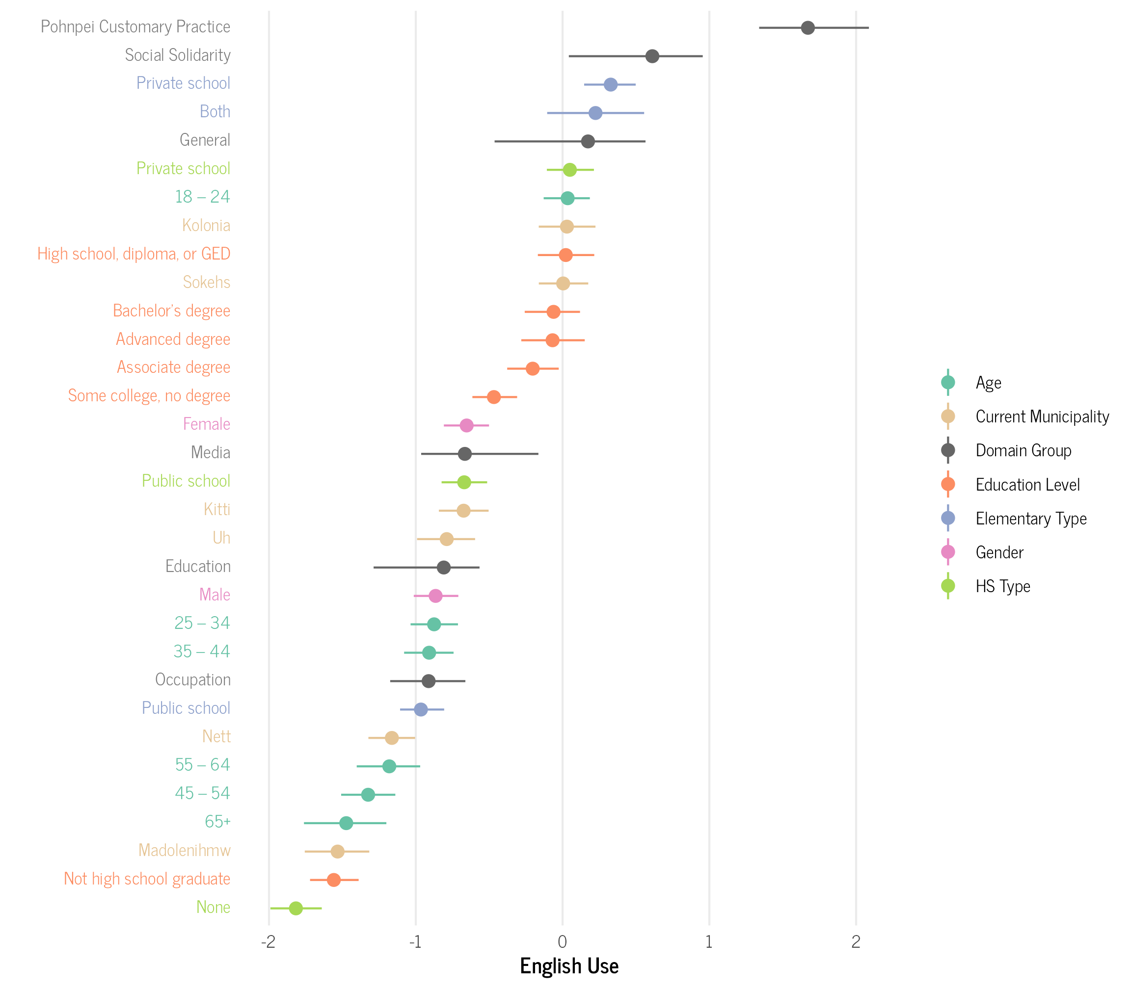
We can now more clearly see which groups find English important in each type of domain. For example, those who attended a private elementary on average find English important for all domain types, except the Pohnpei customary practice ones. One the other hand, those who attended public elementary schools find English important for the occupation, education, and media domains, but not the general, social solidarity, and Pohnpei customary practices domains.
Overall, there is a lot of variation in English language use across the different demographic groups, but the only commonality is that all groups on average find it important to not use English for the Pohnpei Customary Practice domains. There is at least still some situations where English is rarely, if at all, used on Pohnpei!
How do the IRT results compare with the original results?
In my dissertation, I simply summed the number of domains a respondent selected English and used that count as the outcome. I then modeled it using a Bayesian poisson HLM model. The results from that model could only tell me which groups were more likely to have higher counts of selecting English, but not which domains they were likely to use it in or not. The model also weighted each domain equally, so could not account for some domains being easier than others to select English for. The previous model found some similar trends to the new IRT model, but in a much less elegant way, namely (see p. 168 of my dissertation for additional details):
- Age 18–24, more English than the grand mean
- Age 45–54 years old less English than the grand mean
- Age 55–64 years old more English than the grand mean
- Not high school graduate less English than the grand mean
- High school graduate more English than the grand mean
- Bachelor’s degree more English than the grand mean
- Public elementary less English than the grand mean
- Public high school more English than the grand mean
The IRT analysis in this post definitely allows for a more nuanced understanding of the data than my old model!
Extra IRT Diagnostic Graphs
As an extra piece, here is some code for how to create a few common IRT diagnostic plots. Some of the code here is adapted from A. Solomon Kurz’s post, but has been adjusted to properly account for the discrimination values in 2-parameter models.
Item Characteristic Curve (ICC)
ICC plots show the probability of endorsing each item at each latent ability level (\(\theta\)). Items with steeper curves have higher discrimination values, since item discrimination is the slope of the curve. The \(\theta\) value for each item where the probability is 50% is the item’s difficulty value.
icc_data <- as_draws_df(domains_eng_irt) %>%
  # Select relevant parameters
  dplyr::select(.draw, b_eta_Intercept, b_logalpha_Intercept,
                starts_with("r_domain")) %>%
  # Reshape and separate parameters
  pivot_longer(starts_with("r_domain")) %>%
  mutate(
    item = str_extract(name, "(?<=\\[).*?(?=,)"),
    parameter = case_when(
      str_detect(name, "eta") ~ "eta_r",
      str_detect(name, "logalpha") ~ "logalpha_r"
    )
  ) %>%
  dplyr::select(-name) %>%
  pivot_wider(names_from = parameter, values_from = value) %>%
  # Compute IRT parameters
  mutate(
    a_i = exp(b_logalpha_Intercept + logalpha_r),  # Discrimination
    b_i = -(b_eta_Intercept + eta_r)               # Difficulty
  ) %>%
  # Create theta grid
  expand(nesting(.draw, item, a_i, b_i),
         theta = seq(-4, 4, # adjust this range as needed
                     length.out = 200)) %>%
  # Compute response probabilities
  mutate(
    p = plogis(a_i * (theta - b_i))  # 2-PL ICC formula
  )

# Summarize and plot
icc_data %>%
  group_by(theta, item) %>%
  median_qi(p) %>%  # Median and 95% intervals
  ggplot(aes(x = theta, y = p, ymin = .lower, ymax = .upper)) +
  geom_ribbon(alpha = 0.3, fill = "gray70") +
  geom_line(color = "#440154") +
  facet_wrap(~ item) +
  labs(title = "Item Characteristic Curves",
       y = "Probability of Selecting English",
       caption = "Ribbon: 95% credible interval",
       x = expression(theta~("English Use"))) +
  theme_clean() +
  scale_y_continuous(labels = scales::percent)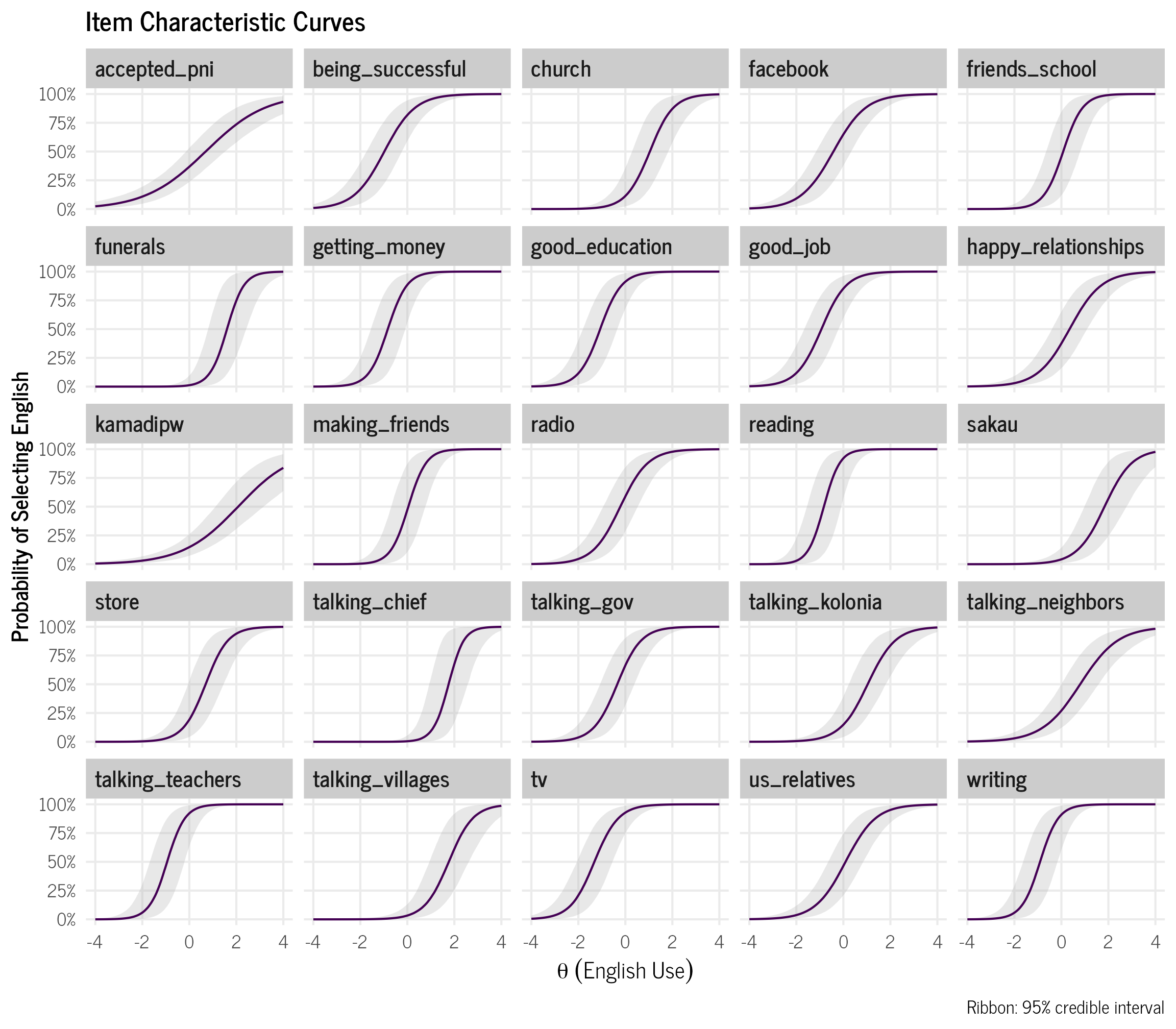
Item Information Curve (IIC)
IIC plots show how much information each individual item provides across the range of \(theta\) values. The Test Information Curve (TIC) in the results section above is simply the sum of the individual IICs and shows how much information the entire instrument provides.
# we use the info data already calculated above

info_data %>%
  group_by(theta, item) %>% # group by theta and item this time
  median_qi(info) %>%  # Use median and quantile intervals
  filter(theta >= -4 & theta <= 4) %>% # limit range to -4 to 4
  ggplot(aes(x = theta,
             y = info,
             ymin = .lower,
             ymax = .upper)) +
  geom_line(linewidth = 0.8) +
  geom_ribbon(alpha = 0.2, colour = NA) +
  labs(
    title = "Item Information Curves",
    x = expression(theta~("English Use")),
    y = "Information",
    caption = "Ribbon: 95% credible interval",
    color = "Item"
  ) +
  facet_wrap(~ item) +
  theme_clean()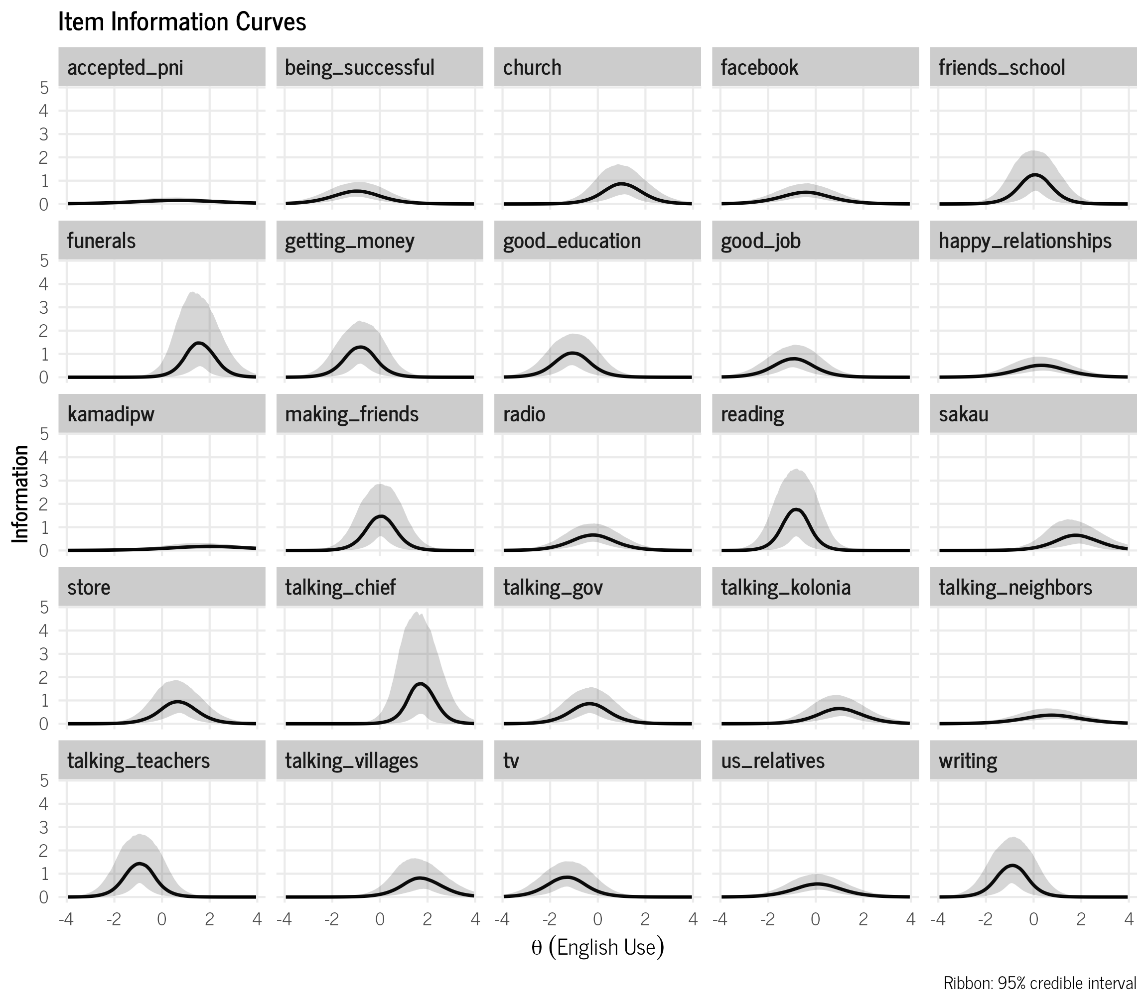
We can also calculate the standard error for each item from the IIC curves.
# we use the info data already calculated above

info_data %>%
  mutate(se = 1 / sqrt(info)) %>%
  group_by(theta, item) %>% # group by theta and item this time
  median_qi(se) %>%  # Use median and quantile intervals
  filter(theta >= -4 & theta <= 4) %>% # limit range to -4 to 4
  ggplot(aes(x = theta,
             y = se,
             ymin = .lower,
             ymax = .upper)) +
  geom_line(linewidth = 0.8) +
  geom_ribbon(alpha = 0.2, colour = NA) +
  labs(
    title = "Item Standard Error Curves",
    x = expression(theta~("English Use")),
    y = "SE",
    caption = "Ribbon: 95% credible interval",
    color = "Item"
  ) +
  facet_wrap(~ item) +
  theme_clean() +
  ylim(c(0,50))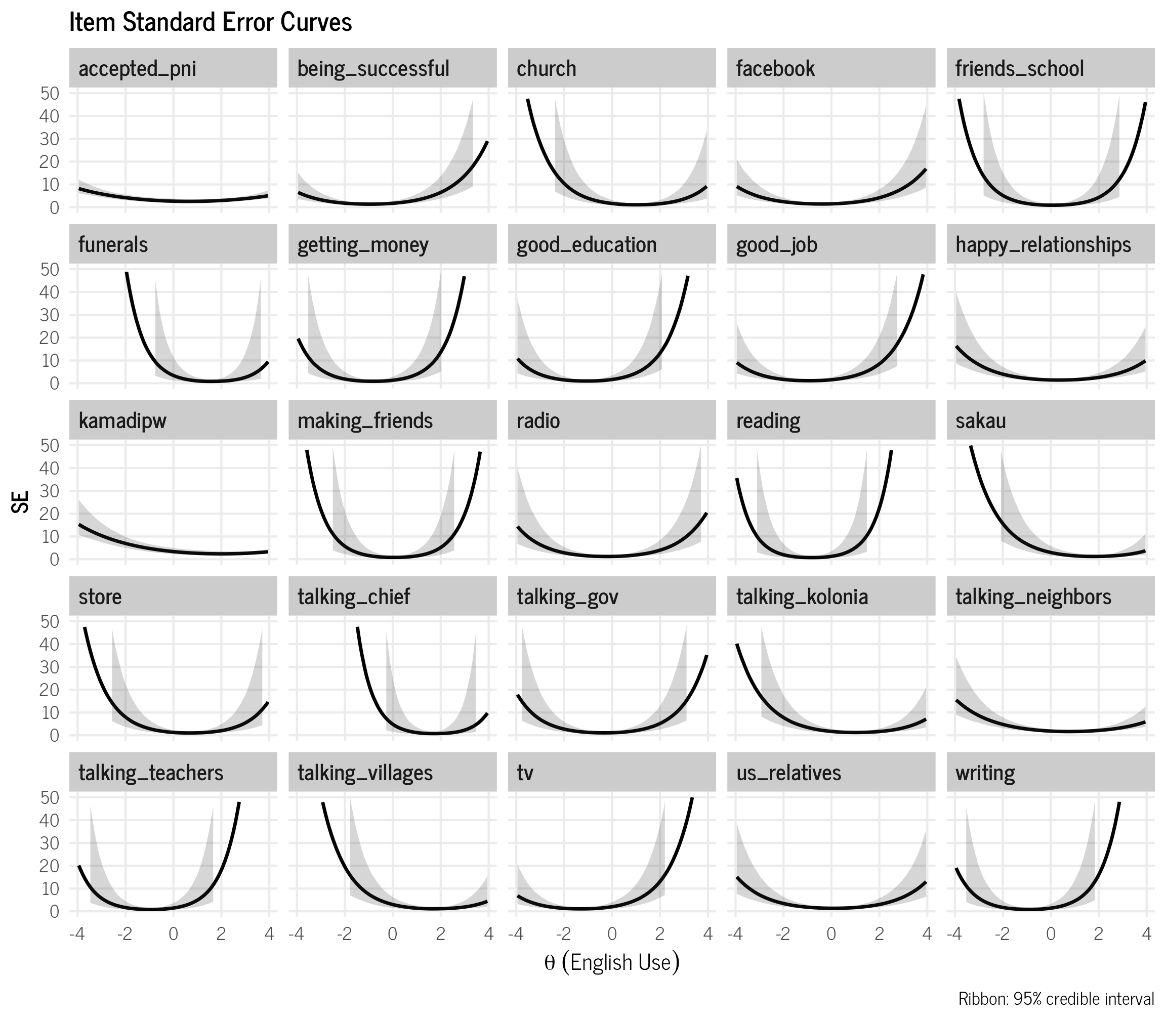
Test Characteristic Curve (TCC)
TCC plots show the expected number of items correct or specific values endorsed for each level of \(\theta\).
tcc_data <- icc_data %>%  # Reuse icc_data from earlier steps
  group_by(.draw, theta) %>%
  summarise(total_score = sum(p),  # Sum probabilities across items
            .groups = "drop") %>%
  group_by(theta) %>%
  median_qi(total_score)  # Get median and uncertainty intervals

ggplot(tcc_data, aes(x = theta, y = total_score)) +
  geom_ribbon(aes(ymin = .lower, ymax = .upper),
              alpha = 0.3, fill = "#2D708E") +
  geom_line(linewidth = 1, color = "#2D708E") +
  labs(title = "Test Characteristic Curve (TCC)",
       x = expression(theta~("English Use")),
       y = "Expected Total Number of English Domains Selected",
       caption = "Ribbon: 95% credible interval") +
  scale_y_continuous(limits = c(0, NA)) +  # Start y-axis at 0
  theme_clean()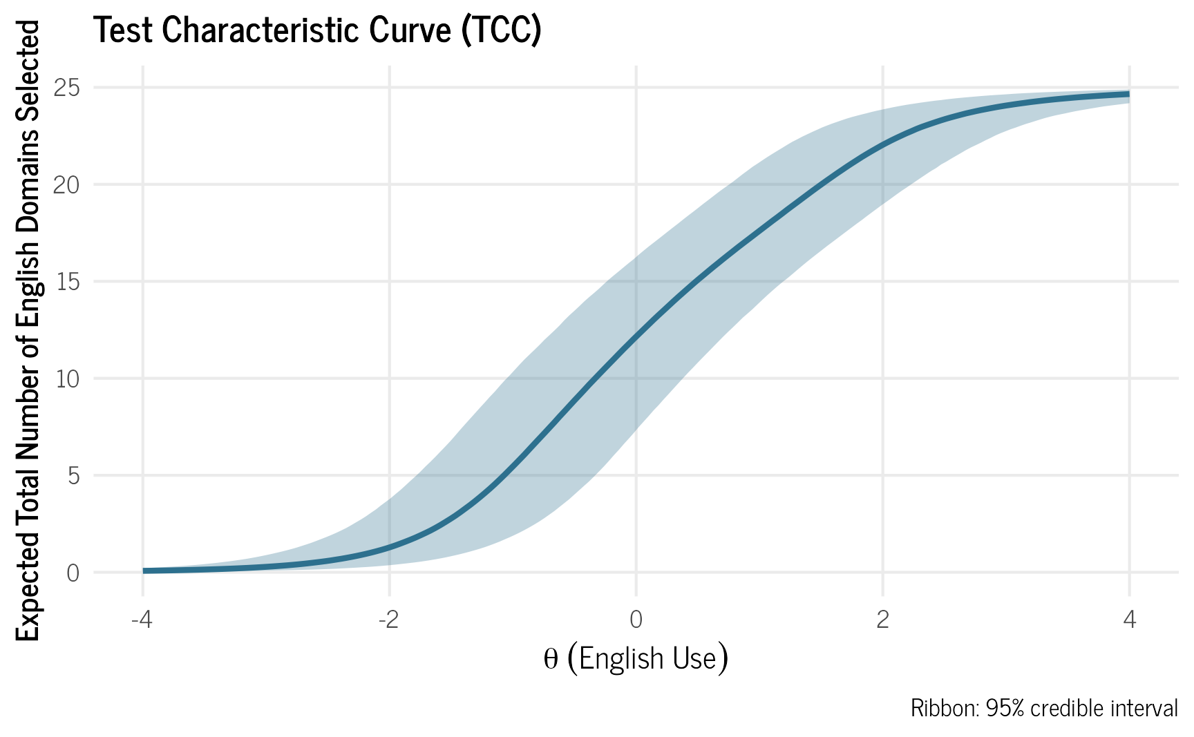
Additional Reading
For additional information about IRT models see:
- https://www.publichealth.columbia.edu/research/population-health-methods/item-response-theory
- https://m-clark.github.io/sem/item-response-theory.html
- https://rpubs.com/fferrero/IRT_Tutorial
- https://www.researchgate.net/profile/Maria-Edelen/publication/6432794_Applying_Item_Response_Theory_IRT_modeling_to_questionnaire_development_evaluation_and_refinement/links/09e415092a186a0ccb000000/Applying-Item-Response-Theory-IRT-modeling-to-questionnaire-development-evaluation-and-refinement.pdf
- https://www.guilford.com/books/The-Theory-and-Practice-of-Item-Response-Theory/R-de-Ayala/9781462547753
Citation
BibTeX citation:
@online{rentz2025,
  author = {Rentz, Bradley},
  title = {Re-Analyzing {Language} {Use} {Data} from {Pohnpei} {Using}
    {Bayesian} {Item} {Response} {Theory} {(IRT)} {Models}},
  date = {2025-04-09},
  url = {https://bradleyrentz.com/blog/2025/04/09/pni-languageuse-irt/},
  langid = {en}
}
For attribution, please cite this work as:
Rentz, B. (2025, April 9). Re-analyzing Language Use Data from
Pohnpei Using Bayesian Item Response Theory (IRT) Models. https://bradleyrentz.com/blog/2025/04/09/pni-languageuse-irt/