
library(tidyverse) # ggplot, dplyr, %>%, and friends
library(janitor) # data cleaning tools
library(brms) # Bayesian models
library(sf) # For importing GIS shapefiles and plotting maps
library(plotly) # Interactive plots
library(tidycensus) # Downloading Census Data
library(naniar) # Visualize missing data
library(geomander) # Matching geographic areas of different sizes
library(spdep) # Identifying neighbors for the CAR models
library(tidybayes) # For Bayesian helper functions
# Custom ggplot theme to make pretty plots
# Get the News Cycle font at https://fonts.google.com/specimen/News+Cycle
theme_clean <- function() {
theme_minimal(base_family = "News Cycle") +
theme(panel.grid.minor = element_blank(),
plot.title = element_text(face = "bold"),
axis.title = element_text(face = "bold"),
strip.text = element_text(face = "bold", size = rel(1), hjust = 0),
strip.background = element_rect(fill = "grey80", color = NA),
legend.title = element_text(face = "bold"))
}Now that the 2024 U.S. presidential election was a few months ago and we are feeling the brunt of the new administration’s actions, it is time to revisit those results to see what new information we can learn.
Hawaiʻi is a solidly blue state, but as some local news sources have reported (see for example this Civil Beat article), the vote share for Trump has risen substantially over time. In this post, I attempt to apply Bayesian Conditional Autoregressive (CAR) Models using brms to try to model the extent of support for Trump across the state among the electorate.
Why use Bayesian CAR models?
Elections are in part spatial phenomena. We know that for a variety of social and historical reasons, one’s geographic community in the U.S. tends to be correlated with one’s race/ethnicity, socioeconomic status, education level, occupation, income, access to government services, health care, and high-quality food, quality of live, and many other factors. Because of that, one’s geographic community is also correlated with one’s political views. We also know that while each community may tend to have specific political views, those political views also influence their neighboring communities and are in turn influenced by their neighbors as well.
Elections then are a measure of a given community’s underlying political views at a specific time. Since we want to know what the underlying views are, we need to create a model that takes into account the spatial (aka community-level) correlation of political views, as well as how nearby communities may influence those views as well.
To take into account the spatial correlations, we’ll use a version of CAR models called the Besag-York-Mollié model that is frequently used to model spatial incidence rates for diseases. This model includes two sets of spatial correlations. First, it models the correlation of a geographic area with all of the areas that border it. Then, it models a random effect for each geographic unit so that it captures the unique variation within each geographic unit.
But before we get too deep into the model, we need to gather the data first.
To get started we will be using these packages.
Prepping HI Election Data
The official precinct-level election results are available from the Hawaiʻi Office of Elections. The election results file contains results for all elections that happened in the state, so we want to import the data and then limit them to only the presidential results.
# import the data directly from the elections site
# need to change the encoding otherwise there will be an error
election_results <- read_csv("https://elections.hawaii.gov/wp-content/results/media.txt",
locale=locale(encoding = "UTF-16LE"),
skip = 1) %>%
# change columns to easier to use names
clean_names() %>%
# remove the final comma in the last column
mutate(in_person_votes = as.numeric(str_replace(in_person_votes,",",""))) %>%
# keep only the presidential results
filter(str_detect(contest_title,"President")==T)
head(election_results)
## # A tibble: 6 × 15
## number_precinct_name split_name precinct_split_id reg_voters ballots reporting contest_id contest_title contest_party choice_id candidate_name choice_party candidate_type mail_votes in_person_votes
## <chr> <chr> <dbl> <dbl> <dbl> <dbl> <dbl> <chr> <lgl> <dbl> <chr> <lgl> <chr> <dbl> <dbl>
## 1 01-01 <NA> 1 6628 4074 1 283 President and Vice President NA 7 "(SL) DE LA CRUZ, Claudia \r\nFor PRESIDENT\r\nGARCIA, Karina \r\nFor VICE PRESIDENT" NA C 18 0
## 2 01-01 <NA> 1 6628 4074 1 283 President and Vice President NA 1 "(D) HARRIS, Kamala D. \r\nFor PRESIDENT\r\nWALZ, Tim \r\nFor VICE PRESIDENT" NA C 2748 0
## 3 01-01 <NA> 1 6628 4074 1 283 President and Vice President NA 5 "(L) OLIVER, Chase \r\nFor PRESIDENT\r\nTER MAAT, Mike \r\nFor VICE PRESIDENT" NA C 35 0
## 4 01-01 <NA> 1 6628 4074 1 283 President and Vice President NA 6 "(S) SONSKI, Peter \r\nFor PRESIDENT\r\nONAK, Lauren\r\nFor VICE PRESIDENT" NA C 4 0
## 5 01-01 <NA> 1 6628 4074 1 283 President and Vice President NA 3 "(G) STEIN, Jill \r\nFor PRESIDENT\r\nWARE, Rudolph\r\nFor VICE PRESIDENT" NA C 63 0
## 6 01-01 <NA> 1 6628 4074 1 283 President and Vice President NA 2 "(R) TRUMP, Donald J. \r\nFor PRESIDENT\r\nVANCE, JD \r\nFor VICE PRESIDENT" NA C 1160 0Now that the data are imported, we need to remove unnecessary columns and convert one row for each candidate per precinct into one row per precinct with the results for each party.
election_results_2024 <- election_results %>%
rename(precinct_name = number_precinct_name) %>%
group_by(precinct_name,contest_id,contest_title,choice_id,candidate_name) %>%
summarise(total_reg_voters = sum(reg_voters),
total_ballots = sum(ballots),
total_votes = sum(mail_votes) + sum(in_person_votes)) %>%
ungroup() %>%
mutate(party = str_extract(candidate_name,"\\((\\w+)\\)",group=1)) %>%
select(precinct_name,contest_title,total_reg_voters:party) %>%
pivot_wider(names_from = party,
values_from = total_votes,
values_fill = 0) %>%
mutate(total_votes = D + R + L + G + S + SL) %>%
select(precinct_name,R,total_votes) %>%
# remove precincts with 0 votes
filter(total_votes > 0 ) %>%
rename(total_votes_2024 = total_votes,
R_2024 = R)
head(election_results_2024)
## # A tibble: 6 × 3
## precinct_name R_2024 total_votes_2024
## <chr> <dbl> <dbl>
## 1 01-01 1289 4240
## 2 01-02 839 2815
## 3 01-03 1144 3903
## 4 02-01 1736 6210
## 5 02-02 67 152
## 6 02-03 1578 5040Let’s quickly look at the results for Trump as a percentage of the total votes.
election_results_2024 %>%
mutate(perc_trump = R_2024 / total_votes_2024) %>%
ggplot(aes(x=reorder(precinct_name,-perc_trump),
y = perc_trump)) +
geom_bar(stat="identity") +
theme_clean() +
theme(axis.text.x = element_blank(),
panel.grid = element_blank()) +
geom_hline(yintercept = 0.5,
linetype = 'dotted',
color = "#009E73") +
ylab("Percent Voted for Trump") +
scale_y_continuous(labels = scales::percent) +
xlab("Precinct") 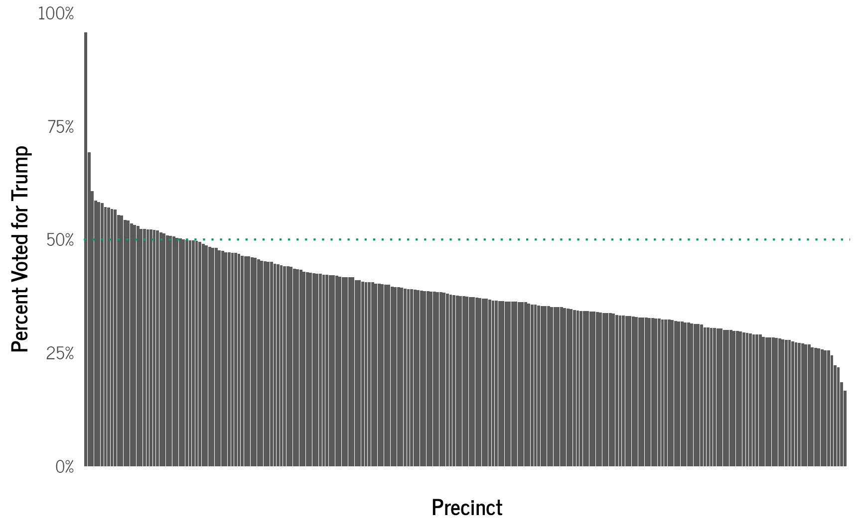
We see that Trump only had 50% or more of the vote in only 31 out of 235 precincts, but had at least 25% of the vote in almost all.
To dig into this more, we need to download the election precinct shape files from the Hawaiʻi Statewide GIS Program and then link the precinct names to the shape file. Now we can create a map to show how each precinct voted.
precincts_shape_2024 <- st_read("data/Election_Precincts.shp", quiet = TRUE)
# join the election results to the shape file
precincts_results_2024 <- precincts_shape_2024 %>%
left_join(election_results_2024, by = c("dp"="precinct_name"))%>%
filter(total_votes_2024 > 0)
election_plot1 <- precincts_results_2024 %>%
mutate(`Percent Trump` = R_2024 / total_votes_2024) %>%
ggplot() +
geom_sf(aes(fill = `Percent Trump`)) +
theme_void() +
scale_fill_gradient2(labels = scales::label_percent(scale=100),
low = "#313695",
high = "#a50026",
midpoint=0.5,
mid = "#ffffbf")
ggplotly(election_plot1)Our First CAR Model
Let’s create our first BYM model to better understand the actual expected level of support for Trump in each election precinct.
First, we need to create a list of neighboring election precincts using the poly2nb() function of the spdep package and then create a weights matrix from the neighbors list with the nb2mat() function. We will also need to unfortunately remove any precincts that do not have any neighbors.
Now we create our first model. This model will only include an intercept and spatial correlations. We will use a negative binomial model since we are modelling count data that may be overdispersed. For the outcome, we will use the number of votes Trump received in each precinct, and we will include a rate() argument to indicate the total number of votes cast in that precinct, since each precinct can vary in the number of actual votes cast. We also need to use the data2 argument to tell brms where to find the neighborhood weight matrix. I am also using more iterations than usual for the model, since the CAR models otherwise tend to have too high r-hat values which indicate poor mixing of the model’s chains.
trump_model <- brm(bf(R_2024 | rate(total_votes_2024) ~ 1 +
car(W, type = "bym2",gr=objectid)), # spatial correlation
data = precincts_results_2024_final,
data2 = list(W=W), # the neighborhood weight matrix
cores=6,
init = 0,
iter = 8000, # need lots of iterations for good convergence
control = list(adapt_delta = 0.9999999999,
max_treedepth=14),
save_pars = save_pars(all = TRUE),
family=negbinomial())At first glance the model seems to have run fine with good r-hat values and the posterior predictive check plots show that we are sampling the outcome fairly well.
summary(trump_model)
## Family: negbinomial
## Links: mu = log; shape = identity
## Formula: R_2024 | rate(total_votes_2024) ~ 1 + car(W, type = "bym2", gr = objectid)
## Data: precincts_results_2024_final (Number of observations: 232)
## Draws: 4 chains, each with iter = 8000; warmup = 4000; thin = 1;
## total post-warmup draws = 16000
##
## Correlation Structures:
## Estimate Est.Error l-95% CI u-95% CI Rhat Bulk_ESS Tail_ESS
## rhocar 1.00 0.00 1.00 1.00 1.01 761 1466
## sdcar 31.82 3.64 24.79 39.21 1.01 736 1276
##
## Regression Coefficients:
## Estimate Est.Error l-95% CI u-95% CI Rhat Bulk_ESS Tail_ESS
## Intercept -0.97 0.01 -0.99 -0.96 1.00 15488 11832
##
## Further Distributional Parameters:
## Estimate Est.Error l-95% CI u-95% CI Rhat Bulk_ESS Tail_ESS
## shape 40410.79 3816295.64 0.15 151.45 1.01 586 1907
##
## Draws were sampled using sampling(NUTS). For each parameter, Bulk_ESS
## and Tail_ESS are effective sample size measures, and Rhat is the potential
## scale reduction factor on split chains (at convergence, Rhat = 1).
pp_check(trump_model)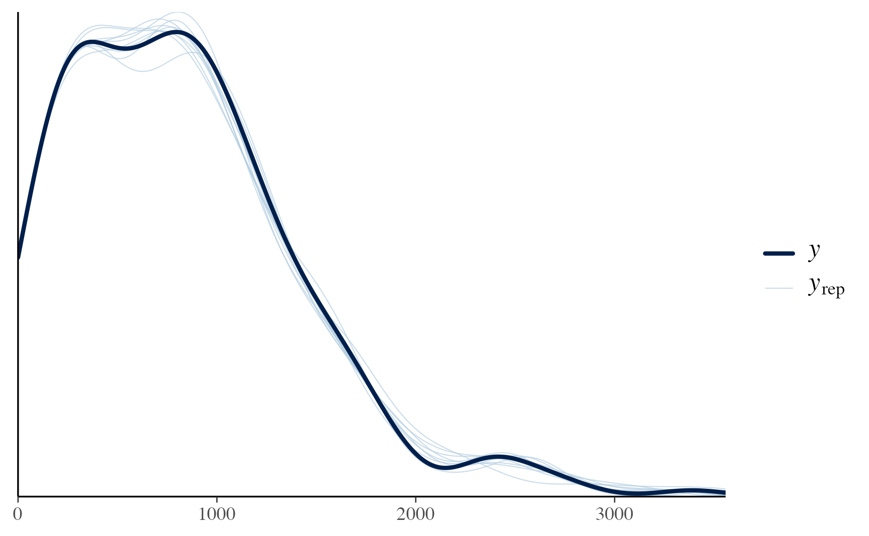
Let’s update our map to see what the expected support for Trump is. First, we need to generate the predicted values for each precinct using predicted_draws() then calculate the median predicted value with median_hdi(). Finally we calculate the expected percentage of votes by using the observed total number of votes and compare that percentage to the observed percentage of votes for Trump.
trump_model_preds <- trump_model %>%
predicted_draws(newdata = precincts_results_2024_final,
ndraws = 1500) %>%
data.frame() %>% # change to df to drop spatial element so can use median_hdi()
group_by(dp) %>%
median_hdi(.prediction)
predicted_percentages_model1 <- precincts_results_2024 %>%
left_join(trump_model_preds) %>%
mutate(`Expected Percentage for Trump` = `.prediction` / total_votes_2024,
`Original Percentage for Trump` = R_2024 / total_votes_2024,
`Change in Percentage for Trump` = `Expected Percentage for Trump` -`Original Percentage for Trump`)
election_plot2 <- predicted_percentages_model1 %>%
ggplot() +
geom_sf(aes(fill = `Expected Percentage for Trump`)) +
theme_void() +
scale_fill_gradient2(labels = scales::label_percent(scale=100),
low = "#313695",
high = "#a50026",
midpoint=0.5,
mid = "#ffffbf")
ggplotly(election_plot2)
election_plot3 <- predicted_percentages_model1 %>%
ggplot() +
geom_sf(aes(fill = `Change in Percentage for Trump`)) +
theme_void() +
scale_fill_gradient2(labels = scales::label_percent(scale=100),
low = "#313695",
high = "#a50026",
midpoint=0,
mid = "#ffffbf")
ggplotly(election_plot3)
predicted_percentages_model1 %>%
ggplot(aes(x=reorder(dp,-`Change in Percentage for Trump`),
y = `Change in Percentage for Trump`)) +
geom_bar(stat="identity") +
theme_clean() +
theme(axis.text.x = element_blank(),
panel.grid = element_blank()) +
ylab("Change in Percentage of Vote for Trump") +
scale_y_continuous(labels = scales::percent) +
xlab("Precinct") 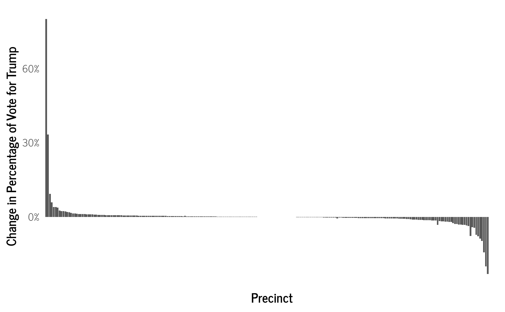
The results show that the vast majority of the precincts have little change from the observed percentage. However, precincts that were strongly in favor of Trump were decreased somewhat, especially those surrounded by precincts with lower support. Similarly, precincts with the lowest number of votes for Trump were increased somewhat. This pattern clearly demonstrates the effects of partial pooling from the random effects of the model, where values are pulled toward the mean, as well as the spatial correlation where values are influenced by their neighbors.
We can also calculate the overall support for Trump across the state by aggregating across the predicted results.
trump_model_votes_overall <- trump_model %>%
predicted_draws(newdata = precincts_results_2024_final,
ndraws = 1500) %>%
data.frame() %>% # change to df to drop spatial element so can use median_hdi()
group_by(`.draw`) %>%
summarize(total_votes_trump_predicted = sum(`.prediction`),
total_votes_overall = sum(total_votes_2024)) %>%
mutate(estimated_percent_trump = total_votes_trump_predicted / total_votes_overall) %>%
ungroup()
trump_model_votes_overall %>%
ggplot(aes(x = estimated_percent_trump)) +
stat_halfeye() +
scale_x_continuous(labels = scales::percent) +
theme_clean() +
ylab("") +
xlab("Estimated Statewide Vote Percentage for Trump")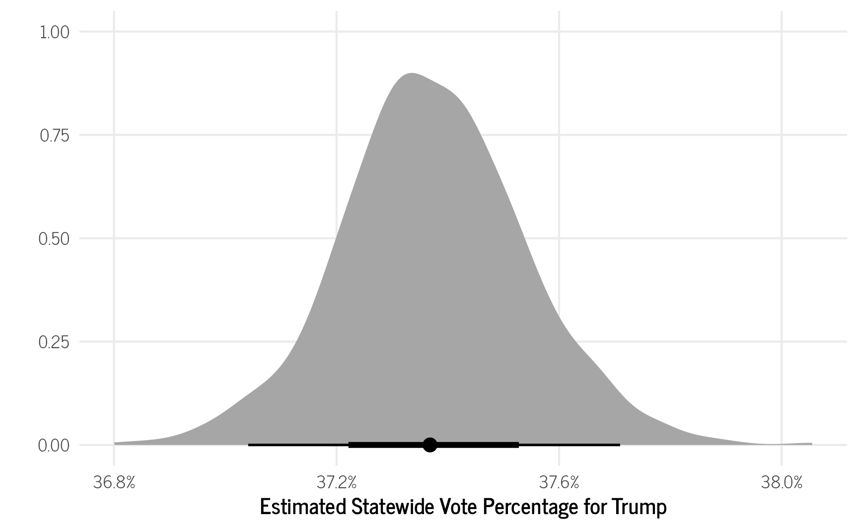
The model predicts that 37.37% of voters statewide supported Trump which is nearly identical to the observed percentage of 37.37% (excluding the three precincts that were removed for not having any neighbors). While our model has the same statewide estimate, it does provide us with two sets of important insights. First, we now have a credible interval for the electoral support for Trump (37.0—37.8%), so that we can specify how certain we are about the level of support for Trump. Second, we have potentially more accurate precinct-level information about the support for Trump.
Now let’s move on to see if we can improve our model by adding additional covariates.
Our Second CAR Model
Our first model only included the spatial correlations and precinct-level effect on the vote. As expected, these did not deviate much from the observed vote results. Now, we want to explore what happens to our model if we add other information about each community, such as education-level, income, age distributions, and other factors that may be correlated with how each community voted.
This task is more challenging since we currently do not have those data available directly for each precinct. To do this, we need to the following steps:
- Download data from the U.S. Census Bureau’s American Community Survey (ACS) for the smallest available geographic unit.
- Match the ACS geographic units to the election precincts.
- Aggregate the ACS data for the election precincts.
Linking the Election Data to Census Data
Since we want to model each communities’ support for Trump, we need to add other information about each community to our model. To do this, we can download block group-level data from the U.S. Census Bureau (assuming those datasets haven’t been removed by the Trump administration by the time you are reading this) and will include a variety of variables from the 2022 American Community Survey that could be associated with how one voted.
acs_data_2022 <- get_acs(geography = "cbg",
state="HI",
year = 2022,
variables = c(total_pop = "B01003_001",
median_age_m = "B01002_002",
median_age_w = "B01002_003",
white_pop = "B02001_002",
asian_pop = "B02001_005",
hi_pi_combo = "B02012_001",
latino = "B03003_001",
no_school = "B15003_002",
hs_diploma = "B15003_017",
ged = "B15003_018",
bachelors = "B15003_022",
masters = "B15003_023",
prof_degree = "B15003_024",
doctorate = "B15003_025",
median_household_income = "B19013_001",
median_rent_gross_income = "B25071_001",
veterans = "B99211_002",
total_occupied = "B25003_001",
total_rented = "B25003_003",
total_households_lang = "C16002_001",
total_asian_pi_lang_lep = "C16002_010",
median_age_men = "B01002_002",
median_age_women = "B01002_003"
)) %>%
pivot_wider(names_from = variable, values_from = c(estimate, moe))
head(acs_data_2022)
## # A tibble: 6 × 44
## GEOID NAME estimate_median_age_m estimate_median_age_w estimate_total_pop estimate_white_pop estimate_asian_pop estimate_hi_pi_combo estimate_latino estimate_no_school estimate_hs_diploma estimate_ged estimate_bachelors estimate_masters estimate_prof_degree estimate_doctorate
## <chr> <chr> <dbl> <dbl> <dbl> <dbl> <dbl> <dbl> <dbl> <dbl> <dbl> <dbl> <dbl> <dbl> <dbl> <dbl>
## 1 150010201001 Block Group 1; Cen… 35.5 44.8 1462 178 450 641 1462 10 286 16 159 71 10 3
## 2 150010201002 Block Group 2; Cen… 49.7 53.3 602 222 125 129 602 0 103 2 169 32 5 9
## 3 150010201003 Block Group 3; Cen… 55.2 56.8 1339 435 272 399 1339 28 255 23 230 50 15 94
## 4 150010201004 Block Group 4; Cen… 34 42.9 1096 146 310 553 1096 0 197 30 94 44 4 9
## 5 150010202021 Block Group 1; Cen… 42 35 1279 584 166 361 1279 0 305 135 157 12 0 26
## 6 150010202022 Block Group 2; Cen… 45.6 44.1 1023 242 328 354 1023 15 171 10 152 48 13 11
## # ℹ 28 more variables: estimate_median_household_income <dbl>, estimate_total_occupied <dbl>, estimate_total_rented <dbl>, estimate_median_rent_gross_income <dbl>, estimate_veterans <dbl>, estimate_total_households_lang <dbl>, estimate_total_asian_pi_lang_lep <dbl>, moe_median_age_m <dbl>,
## # moe_median_age_w <dbl>, moe_total_pop <dbl>, moe_white_pop <dbl>, moe_asian_pop <dbl>, moe_hi_pi_combo <dbl>, moe_latino <dbl>, moe_no_school <dbl>, moe_hs_diploma <dbl>, moe_ged <dbl>, moe_bachelors <dbl>, moe_masters <dbl>, moe_prof_degree <dbl>, moe_doctorate <dbl>,
## # moe_median_household_income <dbl>, moe_total_occupied <dbl>, moe_total_rented <dbl>, moe_median_rent_gross_income <dbl>, moe_veterans <dbl>, moe_total_households_lang <dbl>, moe_total_asian_pi_lang_lep <dbl>Match the ACS Block Groups to Election Precincts
Next, we import the census block group shape files which can also be downloaded from the Hawaiʻi GIS project linked above. However, the problem we face next is that the election precincts and the census block groups comprise different areas. Luckily, we can use the geo_match() function from the geomander package to match the voting precincts to the block groups.
# import census block group shape file
hi_bg_shape_2020 <- st_read("data/hi_bg_2020_bound.shp", quiet = TRUE)
# create some additional variables for the ACS data
acs_data_2022_prepped <- acs_data_2022 %>%
rename_with( ~gsub("estimate_","", .x)) %>%
mutate(hs_ged = ged + hs_diploma,
percent_asian_pi_lang_lep = total_asian_pi_lang_lep/total_households_lang) %>%
select(-latino,
-ged,
-hs_diploma, -total_asian_pi_lang_lep,
-total_households_lang) %>%
filter(total_pop > 0)
# link to census block shape
acs_data_2022_prepped_geo <- hi_bg_shape_2020 %>%
inner_join(acs_data_2022_prepped, by = c("GEOID20"="GEOID"))
# match precincts to block groups
matches_2024 <- geo_match(from = acs_data_2022_prepped_geo,
to = precincts_results_2024,
method = 'centroid')
acs_data_2022_prepped_geo$match_id_2024 <- matches_2024
precincts_results_2024$match_id_2024 <- 1:nrow(precincts_results_2024)Aggregating ACS Block Group Results to Election Precincts
After matching the precincts to the census block groups, the values from the smaller sized block groups need to be aggregated up to the larger election precincts using the estimate_up() function. This only directly works with counts. For continuous values, we will calculate the median for all the block groups within each precinct. There may be a better way to do that, but we’ll use that for now. One additional limitation of aggregating the census results is that we lose the ability to use the ACS’s reported measurement error values in the model, which means our model may be more confident in the ACS values than it otherwise should be. There may be ways to aggregate the measurement errors (such as this guide from the U.S. Census Bureau), but I need to dig further into it later to figure it out and may make a new blog post about it.
# list the variables to estimate up
vars <- c("total_pop", "white_pop", "asian_pop", "hi_pi_combo",
"no_school", "hs_ged", "bachelors", "masters",
"prof_degree", "doctorate", "veterans")
# create new copy of the precinct data
precincts_results_2024_acs <- precincts_results_2024
# estimate up the results from the census block group to the precinct.
for (var in vars) {
col_name <- paste0(var, "_acs")
precincts_results_2024_acs[[col_name]] <- estimate_up(
value = acs_data_2022_prepped_geo[[var]],
group = matches_2024
)
}
acs_2022_continuous <- acs_data_2022_prepped_geo %>%
data.frame() %>%
select(-geometry) %>%
group_by(match_id_2024) %>%
summarise(median_household_income_acs = median(median_household_income, na.rm=T),
median_rent_gross_income_acs = median(median_rent_gross_income, na.rm = T),
median_age_men_acs = median(median_age_m, na.rm = T),
median_age_women_acs = median(median_age_w, na.rm=T)) %>%
ungroup()
model2_data <- precincts_results_2024_acs %>%
left_join(acs_2022_continuous) %>%
dplyr::select(-zeropop)It looks like the continuous ACS variables have a fair amount of missingness. We will need to impute those data in our final model later.
# visualize missing data
gg_miss_var(model2_data) + theme_clean()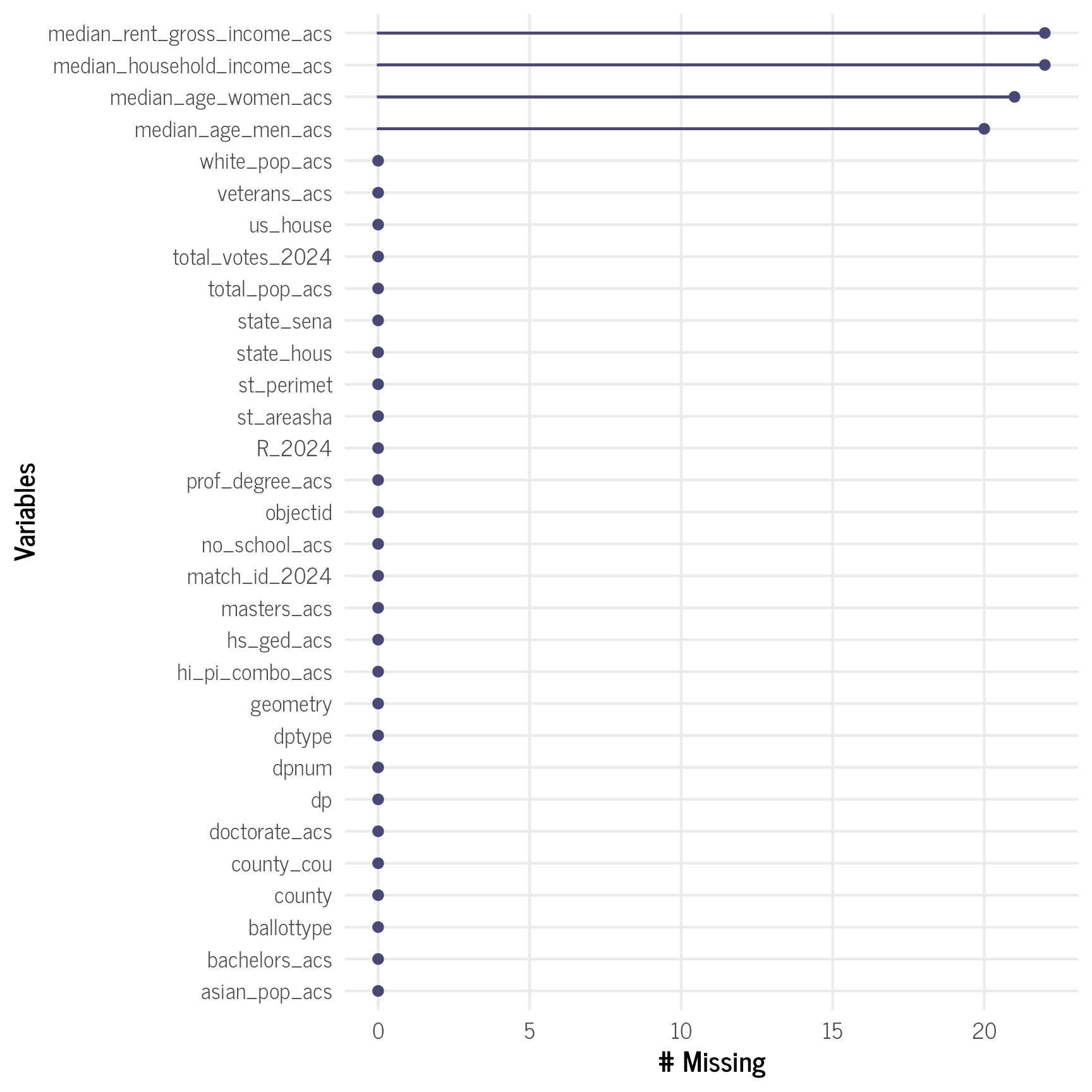
Building Our Second Model
For our second model, we include all the ACS variables, but for the ones with missing values, we will impute the missing values with the mi() function in the model itself. To be safe, we will use the skew_normal() distribution for the imputation formulae’s families, since the underlying distribution may be somewhat skewed. We also standardized all the predictors in the model to make it easier to compare the results between predictors and easier to set priors for them.
# remove precincts with no neighbors
model2_data_final <- model2_data %>%
filter(grepl("67|73|94",objectid) == FALSE) %>%
# standardize the predictors
mutate(across(ends_with("_acs"), ~ as.numeric(scale(.x,
center = TRUE,
scale = TRUE))))
# set prior for the betas
priors <- prior(normal(0,3), class = "b")
# set the formulae
votes <- bf(R_2024 | rate(total_votes_2024) ~ white_pop_acs +
asian_pop_acs +
hi_pi_combo_acs +
no_school_acs +
hs_ged_acs +
bachelors_acs +
masters_acs +
prof_degree_acs +
doctorate_acs +
veterans_acs +
mi(median_household_income_acs) +
mi(median_age_men_acs) +
mi(median_age_women_acs) +
mi(median_rent_gross_income_acs) +
car(W, type = "bym2",gr=objectid)) + negbinomial()
mi_income <- bf(median_household_income_acs | mi() ~ white_pop_acs +
asian_pop_acs +
hi_pi_combo_acs +
no_school_acs +
hs_ged_acs +
bachelors_acs +
masters_acs +
prof_degree_acs +
doctorate_acs +
veterans_acs) + skew_normal()
mi_rent <- bf(median_rent_gross_income_acs | mi() ~ white_pop_acs +
asian_pop_acs +
hi_pi_combo_acs +
no_school_acs +
hs_ged_acs +
bachelors_acs +
masters_acs +
prof_degree_acs +
doctorate_acs +
veterans_acs) + skew_normal()
mi_age_men <- bf(median_age_men_acs | mi() ~ white_pop_acs +
asian_pop_acs +
hi_pi_combo_acs +
no_school_acs +
hs_ged_acs +
bachelors_acs +
masters_acs +
prof_degree_acs +
doctorate_acs +
veterans_acs) + skew_normal()
mi_age_women <- bf(median_age_women_acs | mi() ~ white_pop_acs +
asian_pop_acs +
hi_pi_combo_acs +
no_school_acs +
hs_ged_acs +
bachelors_acs +
masters_acs +
prof_degree_acs +
doctorate_acs +
veterans_acs) + skew_normal()
# put it all together in the model
trump_model2 <- brm(votes + mi_income + mi_rent + mi_age_men + mi_age_women + set_rescor(FALSE),
data = model2_data_final,
data2 = list(W=W),
cores=6,
chains = 4,
init = 0,
iter = 8000,
control = list(adapt_delta = 0.9999999999,
max_treedepth=14),
prior=priors)The model summary indicates that we have good r-hats, and the posterior predictive plot shows good sampling of the main outcome variable. The coefficients of the predictors for the number of votes for Trump are quite small, but there are some expected trends:
- The larger the population of individuals with bachelors or doctorate degrees as their highest educational attainment, the lower the number of votes for Trump.
- The larger the population of veterans, the more votes for Trump there were.
- Larger white and Hawaiian/Pacific Islander populations were somewhat associated with more votes for Trump.
- There was no association between larger Asian populations and changes in the number of votes for Trump.
summary(trump_model2)
## Family: MV(negbinomial, skew_normal, skew_normal, skew_normal, skew_normal)
## Links: mu = log; shape = identity
## mu = identity; sigma = identity; alpha = identity
## mu = identity; sigma = identity; alpha = identity
## mu = identity; sigma = identity; alpha = identity
## mu = identity; sigma = identity; alpha = identity
## Formula: R_2024 | rate(total_votes_2024) ~ white_pop_acs + asian_pop_acs + hi_pi_combo_acs + no_school_acs + hs_ged_acs + bachelors_acs + masters_acs + prof_degree_acs + doctorate_acs + veterans_acs + mi(median_household_income_acs) + mi(median_age_men_acs) + mi(median_age_women_acs) + mi(median_rent_gross_income_acs) + car(W, type = "bym2", gr = objectid)
## median_household_income_acs | mi() ~ white_pop_acs + asian_pop_acs + hi_pi_combo_acs + no_school_acs + hs_ged_acs + bachelors_acs + masters_acs + prof_degree_acs + doctorate_acs + veterans_acs
## median_rent_gross_income_acs | mi() ~ white_pop_acs + asian_pop_acs + hi_pi_combo_acs + no_school_acs + hs_ged_acs + bachelors_acs + masters_acs + prof_degree_acs + doctorate_acs + veterans_acs
## median_age_men_acs | mi() ~ white_pop_acs + asian_pop_acs + hi_pi_combo_acs + no_school_acs + hs_ged_acs + bachelors_acs + masters_acs + prof_degree_acs + doctorate_acs + veterans_acs
## median_age_women_acs | mi() ~ white_pop_acs + asian_pop_acs + hi_pi_combo_acs + no_school_acs + hs_ged_acs + bachelors_acs + masters_acs + prof_degree_acs + doctorate_acs + veterans_acs
## Data: model2_data_final (Number of observations: 232)
## Draws: 4 chains, each with iter = 8000; warmup = 4000; thin = 1;
## total post-warmup draws = 16000
##
## Correlation Structures:
## Estimate Est.Error l-95% CI u-95% CI Rhat Bulk_ESS Tail_ESS
## rhocar_R2024 1.00 0.00 1.00 1.00 1.00 872 1855
## sdcar_R2024 25.35 2.78 19.94 30.87 1.00 898 1860
##
## Regression Coefficients:
## Estimate Est.Error l-95% CI u-95% CI Rhat Bulk_ESS Tail_ESS
## R2024_Intercept -0.98 0.00 -0.99 -0.97 1.00 13372 12172
## medianhouseholdincomeacs_Intercept -0.00 0.06 -0.12 0.12 1.00 19311 12746
## medianrentgrossincomeacs_Intercept -0.02 0.07 -0.14 0.12 1.00 17371 13008
## medianagemenacs_Intercept -0.01 0.06 -0.13 0.11 1.00 19563 11729
## medianagewomenacs_Intercept -0.01 0.06 -0.12 0.11 1.00 19280 12170
## R2024_white_pop_acs 0.01 0.02 -0.02 0.05 1.00 4100 6713
## R2024_asian_pop_acs -0.00 0.02 -0.05 0.05 1.00 3958 6013
## R2024_hi_pi_combo_acs 0.01 0.02 -0.02 0.05 1.00 3894 7058
## R2024_no_school_acs 0.01 0.01 -0.01 0.03 1.00 6499 8912
## R2024_hs_ged_acs 0.01 0.02 -0.03 0.06 1.00 4290 7310
## R2024_bachelors_acs -0.05 0.02 -0.09 -0.00 1.00 5513 8648
## R2024_masters_acs -0.00 0.02 -0.03 0.03 1.00 6230 9722
## R2024_prof_degree_acs 0.01 0.01 -0.02 0.03 1.00 7238 8662
## R2024_doctorate_acs -0.03 0.01 -0.05 -0.01 1.00 4790 9026
## R2024_veterans_acs 0.03 0.01 0.00 0.05 1.00 6422 10387
## medianhouseholdincomeacs_white_pop_acs -0.05 0.15 -0.36 0.24 1.00 6336 8801
## medianhouseholdincomeacs_asian_pop_acs 0.26 0.24 -0.20 0.73 1.00 6140 8407
## medianhouseholdincomeacs_hi_pi_combo_acs 0.15 0.16 -0.18 0.47 1.00 6503 9378
## medianhouseholdincomeacs_no_school_acs -0.30 0.09 -0.48 -0.13 1.00 18251 11778
## medianhouseholdincomeacs_hs_ged_acs -0.73 0.23 -1.18 -0.28 1.00 7283 9839
## medianhouseholdincomeacs_bachelors_acs 0.03 0.24 -0.44 0.49 1.00 8040 10202
## medianhouseholdincomeacs_masters_acs 0.18 0.15 -0.12 0.48 1.00 16654 11074
## medianhouseholdincomeacs_prof_degree_acs 0.10 0.11 -0.11 0.31 1.00 15549 12643
## medianhouseholdincomeacs_doctorate_acs -0.11 0.10 -0.32 0.09 1.00 16500 12191
## medianhouseholdincomeacs_veterans_acs 0.50 0.12 0.26 0.73 1.00 13380 12695
## medianrentgrossincomeacs_white_pop_acs 0.41 0.15 0.12 0.69 1.00 6181 8867
## medianrentgrossincomeacs_asian_pop_acs 0.10 0.23 -0.35 0.56 1.00 5968 8599
## medianrentgrossincomeacs_hi_pi_combo_acs 0.03 0.15 -0.28 0.33 1.00 6679 9745
## medianrentgrossincomeacs_no_school_acs -0.04 0.09 -0.21 0.13 1.00 16028 11545
## medianrentgrossincomeacs_hs_ged_acs 0.05 0.21 -0.37 0.46 1.00 7700 9519
## medianrentgrossincomeacs_bachelors_acs -0.02 0.22 -0.45 0.40 1.00 8459 10904
## medianrentgrossincomeacs_masters_acs -0.01 0.14 -0.29 0.26 1.00 18008 11908
## medianrentgrossincomeacs_prof_degree_acs -0.13 0.10 -0.33 0.06 1.00 13946 12169
## medianrentgrossincomeacs_doctorate_acs 0.10 0.10 -0.10 0.27 1.00 14128 12458
## medianrentgrossincomeacs_veterans_acs -0.13 0.12 -0.37 0.10 1.00 12775 12132
## medianagemenacs_white_pop_acs -0.72 0.15 -1.01 -0.43 1.00 6004 8307
## medianagemenacs_asian_pop_acs -0.90 0.24 -1.37 -0.44 1.00 5472 8470
## medianagemenacs_hi_pi_combo_acs -0.72 0.16 -1.04 -0.40 1.00 6211 8547
## medianagemenacs_no_school_acs 0.06 0.09 -0.12 0.23 1.00 17858 11684
## medianagemenacs_hs_ged_acs 0.90 0.22 0.47 1.34 1.00 7228 10047
## medianagemenacs_bachelors_acs 0.50 0.23 0.05 0.96 1.00 8249 10228
## medianagemenacs_masters_acs 0.21 0.16 -0.09 0.51 1.00 19368 11762
## medianagemenacs_prof_degree_acs 0.36 0.10 0.16 0.56 1.00 15403 11998
## medianagemenacs_doctorate_acs -0.08 0.10 -0.27 0.11 1.00 15669 11500
## medianagemenacs_veterans_acs 0.09 0.12 -0.15 0.33 1.00 14346 12536
## medianagewomenacs_white_pop_acs -0.83 0.14 -1.12 -0.55 1.00 6011 8271
## medianagewomenacs_asian_pop_acs -0.85 0.23 -1.30 -0.41 1.00 5840 8647
## medianagewomenacs_hi_pi_combo_acs -0.78 0.16 -1.09 -0.47 1.00 6658 9491
## medianagewomenacs_no_school_acs 0.12 0.08 -0.04 0.29 1.00 17341 11413
## medianagewomenacs_hs_ged_acs 0.87 0.22 0.44 1.29 1.00 7368 8602
## medianagewomenacs_bachelors_acs 0.47 0.23 0.03 0.91 1.00 8053 10408
## medianagewomenacs_masters_acs 0.21 0.15 -0.09 0.51 1.00 18030 11824
## medianagewomenacs_prof_degree_acs 0.37 0.10 0.17 0.58 1.00 15445 12168
## medianagewomenacs_doctorate_acs -0.04 0.09 -0.22 0.14 1.00 15854 11385
## medianagewomenacs_veterans_acs 0.07 0.11 -0.15 0.30 1.00 15030 12514
## R2024_mimedian_household_income_acs -0.00 0.01 -0.02 0.02 1.00 4329 7537
## R2024_mimedian_age_men_acs -0.01 0.01 -0.03 0.01 1.00 5165 9254
## R2024_mimedian_age_women_acs -0.05 0.01 -0.07 -0.03 1.00 6081 8865
## R2024_mimedian_rent_gross_income_acs 0.00 0.01 -0.01 0.01 1.00 8156 9983
##
## Further Distributional Parameters:
## Estimate Est.Error l-95% CI u-95% CI Rhat Bulk_ESS Tail_ESS
## shape_R2024 12407.08 1333717.77 0.20 98.56 1.00 938 2421
## sigma_medianhouseholdincomeacs 0.89 0.05 0.80 0.98 1.00 17257 12040
## sigma_medianrentgrossincomeacs 0.96 0.05 0.86 1.07 1.00 13041 10821
## sigma_medianagemenacs 0.89 0.05 0.81 0.99 1.00 16259 11085
## sigma_medianagewomenacs 0.85 0.04 0.77 0.94 1.00 18196 11561
## alpha_medianhouseholdincomeacs 1.06 0.97 -0.88 2.77 1.00 11882 13598
## alpha_medianrentgrossincomeacs 3.14 0.82 1.82 5.03 1.00 13626 9513
## alpha_medianagemenacs 1.21 0.85 -0.70 2.61 1.00 10507 13498
## alpha_medianagewomenacs 0.03 0.82 -1.48 1.44 1.00 16721 14375
##
## Draws were sampled using sampling(NUTS). For each parameter, Bulk_ESS
## and Tail_ESS are effective sample size measures, and Rhat is the potential
## scale reduction factor on split chains (at convergence, Rhat = 1).
pp_check(trump_model2, resp = "R2024")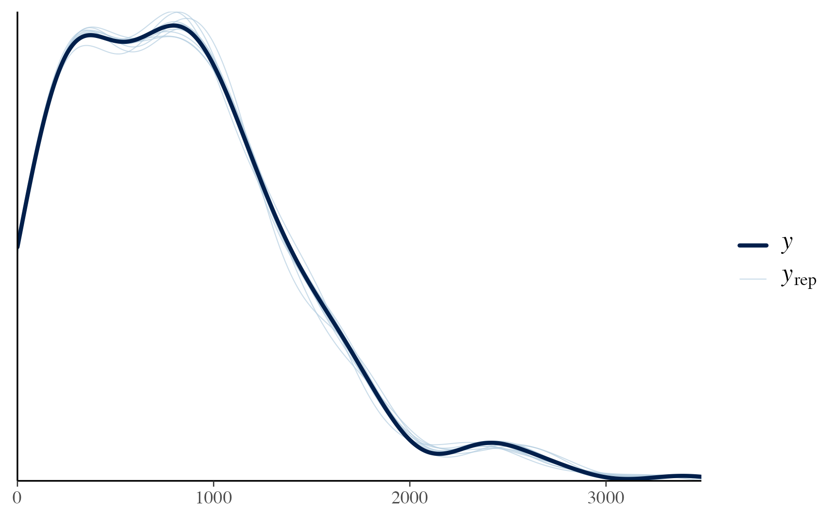
Examining the Predicted Results
To examine the predicted results, we first have to determine the imputed values for those variables that had missing data, then use that dataset to calculate the final predicted values for each election precinct.
# get the imputed values first
data_imputed <- trump_model2 %>%
predicted_draws(newdata = model2_data_final,
ndraws = 1500) %>%
data.frame() %>%
select(-.row:-.draw) %>%
dplyr::filter(`.category` != "R2024") %>%
pivot_wider(names_from = .category,
values_from = .prediction,
values_fn = median) %>%
mutate(median_household_income_acs = case_when(
is.na(median_household_income_acs) == TRUE ~ medianhouseholdincomeacs,
.default = median_household_income_acs
),
median_rent_gross_income_acs = case_when(
is.na(median_rent_gross_income_acs) == TRUE ~ medianrentgrossincomeacs,
.default = median_rent_gross_income_acs
),
median_age_men_acs = case_when(
is.na(median_age_men_acs) == TRUE ~ medianagemenacs,
.default = median_age_men_acs
),
median_age_women_acs = case_when(
is.na(median_age_women_acs) == TRUE ~ medianagewomenacs,
.default = median_age_women_acs
)
)
trump_model_preds2 <- trump_model2 %>%
predicted_draws(newdata = data_imputed,
ndraws = 1500) %>%
data.frame() %>% # change to df to drop spatial element so can use median_hdi()
filter(.category == "R2024") %>%
group_by(dp) %>%
median_hdi(.prediction)
predicted_percentages_model2 <- model2_data_final %>%
left_join(trump_model_preds2) %>%
mutate(`Expected Percentage for Trump` = `.prediction` / total_votes_2024,
`Original Percentage for Trump` = R_2024 / total_votes_2024,
`Change in Percentage for Trump` = `Expected Percentage for Trump` -`Original Percentage for Trump`)
election_plot2_1 <- predicted_percentages_model2 %>%
ggplot() +
geom_sf(aes(fill = `Expected Percentage for Trump`)) +
theme_void() +
scale_fill_gradient2(labels = scales::label_percent(scale=100),
low = "#313695",
high = "#a50026",
midpoint=0.5,
mid = "#ffffbf")
election_plot2_1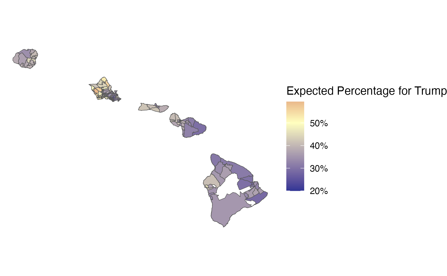
# zoom in on oahu
predicted_percentages_model2 %>%
filter(county == "OAHU") %>%
ggplot() +
geom_sf(aes(fill = `Expected Percentage for Trump`)) +
theme_void() +
scale_fill_gradient2(labels = scales::label_percent(scale=100),
low = "#313695",
high = "#a50026",
midpoint=0.5,
mid = "#ffffbf")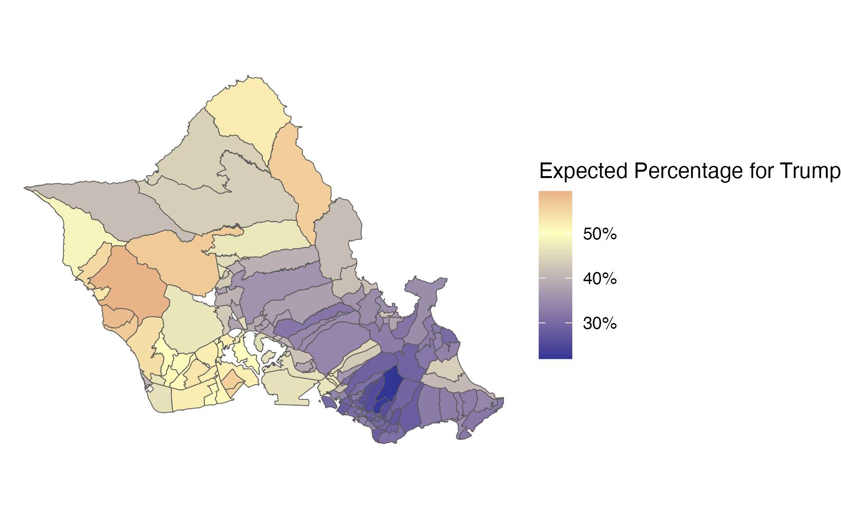
election_plot2_2 <- predicted_percentages_model2 %>%
ggplot() +
geom_sf(aes(fill = `Change in Percentage for Trump`)) +
theme_void() +
scale_fill_gradient2(labels = scales::label_percent(scale=100),
low = "#313695",
high = "#a50026",
midpoint=0,
mid = "#ffffbf")
election_plot2_2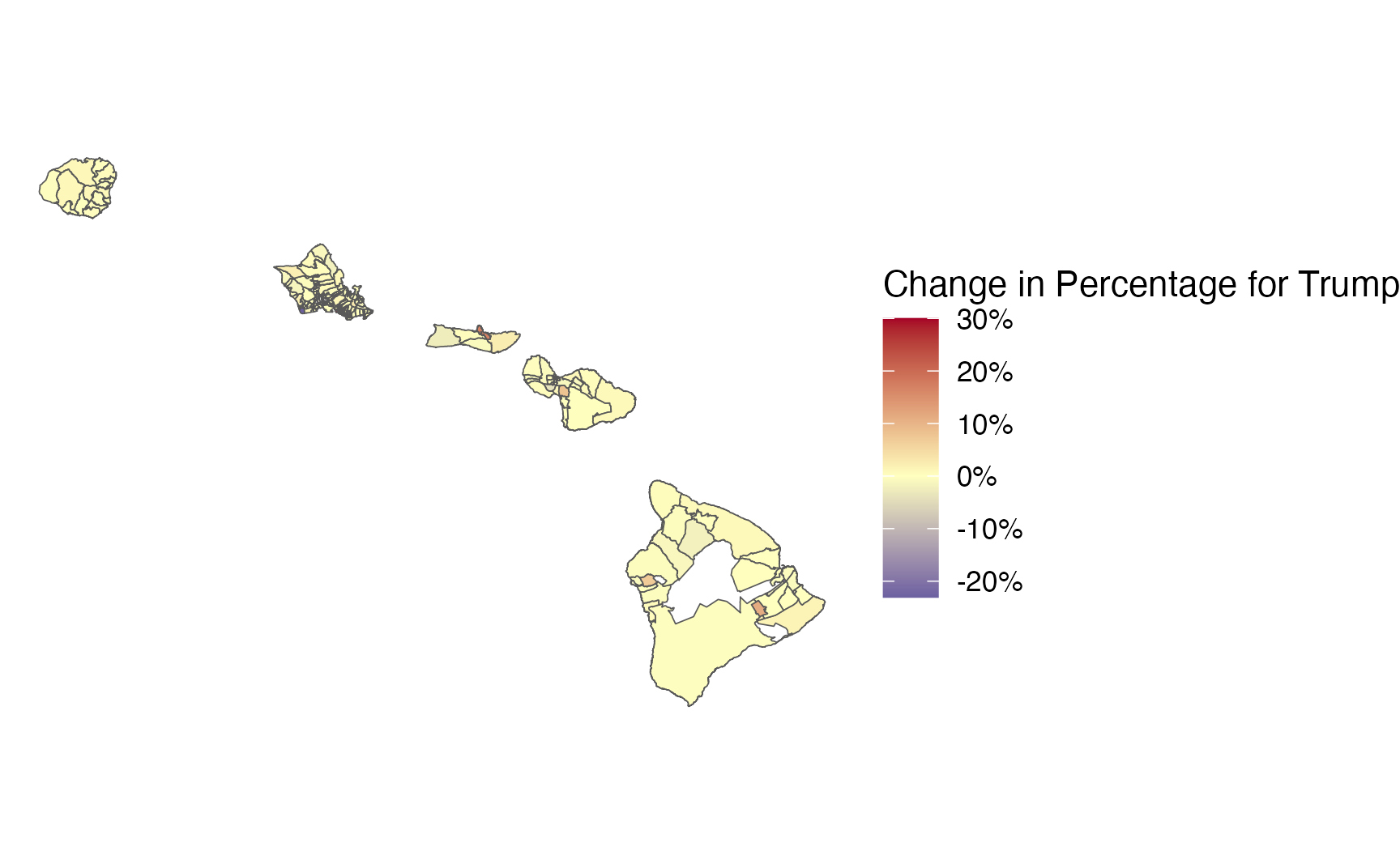
# zoom in on oahu
predicted_percentages_model2 %>%
filter(county == "OAHU") %>%
ggplot() +
geom_sf(aes(fill = `Change in Percentage for Trump`)) +
theme_void() +
scale_fill_gradient2(labels = scales::label_percent(scale=100),
low = "#313695",
high = "#a50026",
midpoint=0,
mid = "#ffffbf")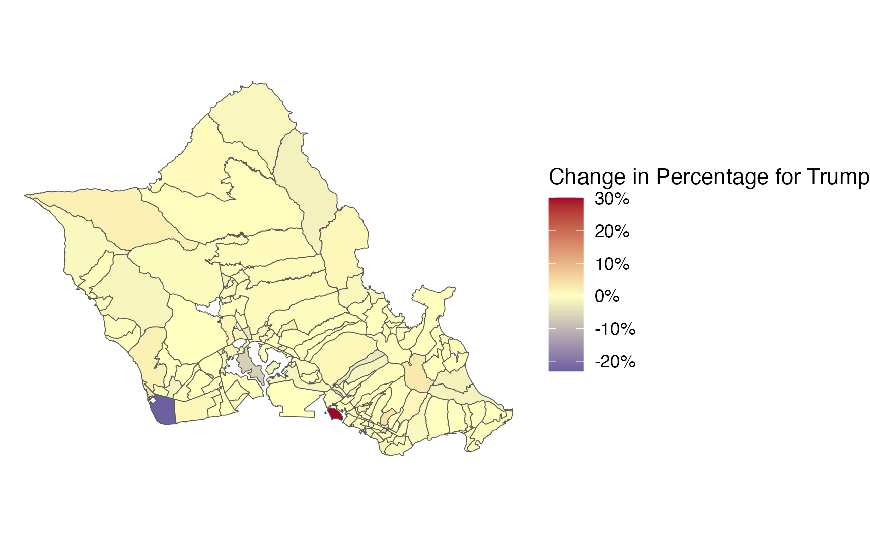
predicted_percentages_model2 %>%
ggplot(aes(x=reorder(dp,-`Change in Percentage for Trump`),
y = `Change in Percentage for Trump`)) +
geom_bar(stat="identity") +
theme_clean() +
theme(axis.text.x = element_blank(),
panel.grid = element_blank()) +
ylab("Change in Percentage of Vote for Trump") +
scale_y_continuous(labels = scales::percent) +
xlab("Precinct")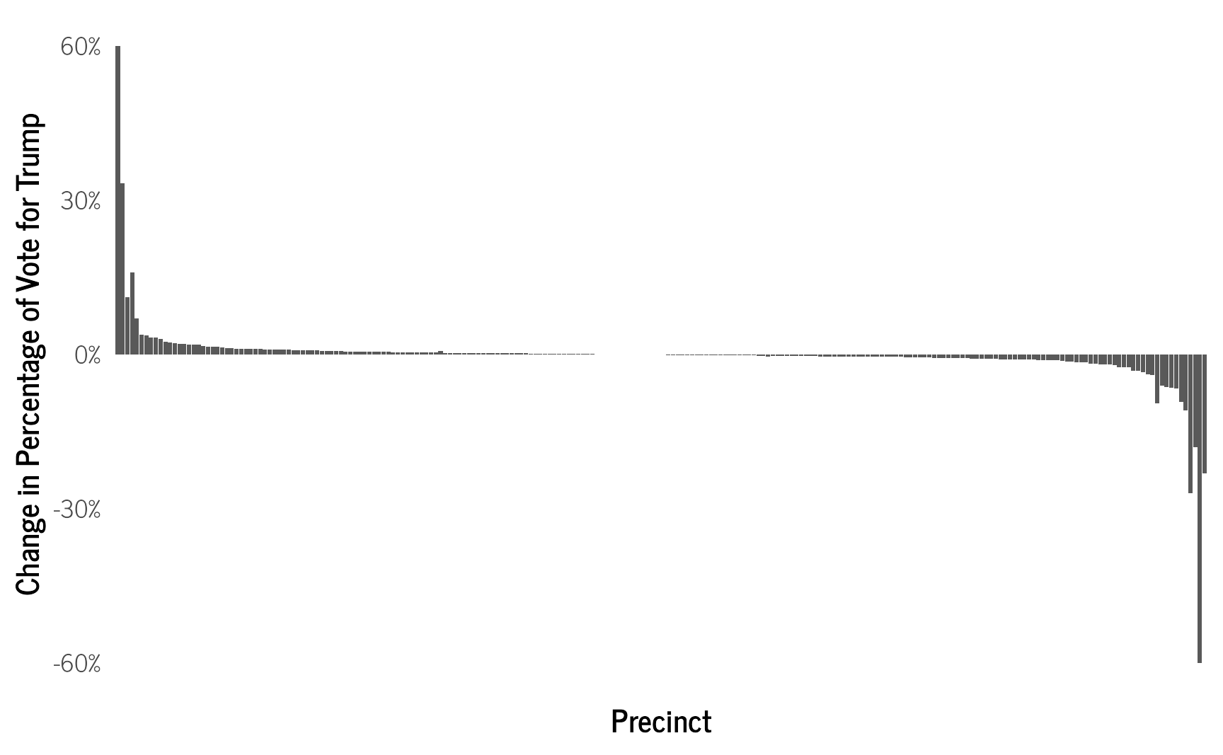
This new model leads to slightly larger changes in the predicted number of votes for Trump among precincts, since we now have other covariates that influence how the model calculates the predicted number of votes.
trump_model_votes_overall2 <- trump_model2 %>%
predicted_draws(newdata = data_imputed,
ndraws = 1500) %>%
data.frame() %>% # change to df to drop spatial element so can use median_hdi()
filter(.category == "R2024") %>%
group_by(`.draw`) %>%
summarize(total_votes_trump_predicted = sum(`.prediction`,na.rm = TRUE),
total_votes_overall = sum(total_votes_2024,na.rm = TRUE)) %>%
mutate(estimated_percent_trump = total_votes_trump_predicted / total_votes_overall) %>%
ungroup()
trump_model_votes_overall2 %>%
ggplot(aes(x = estimated_percent_trump)) +
stat_halfeye() +
scale_x_continuous(labels = scales::percent) +
theme_clean() +
ylab("") +
xlab("Estimated Statewide Vote Percentage for Trump")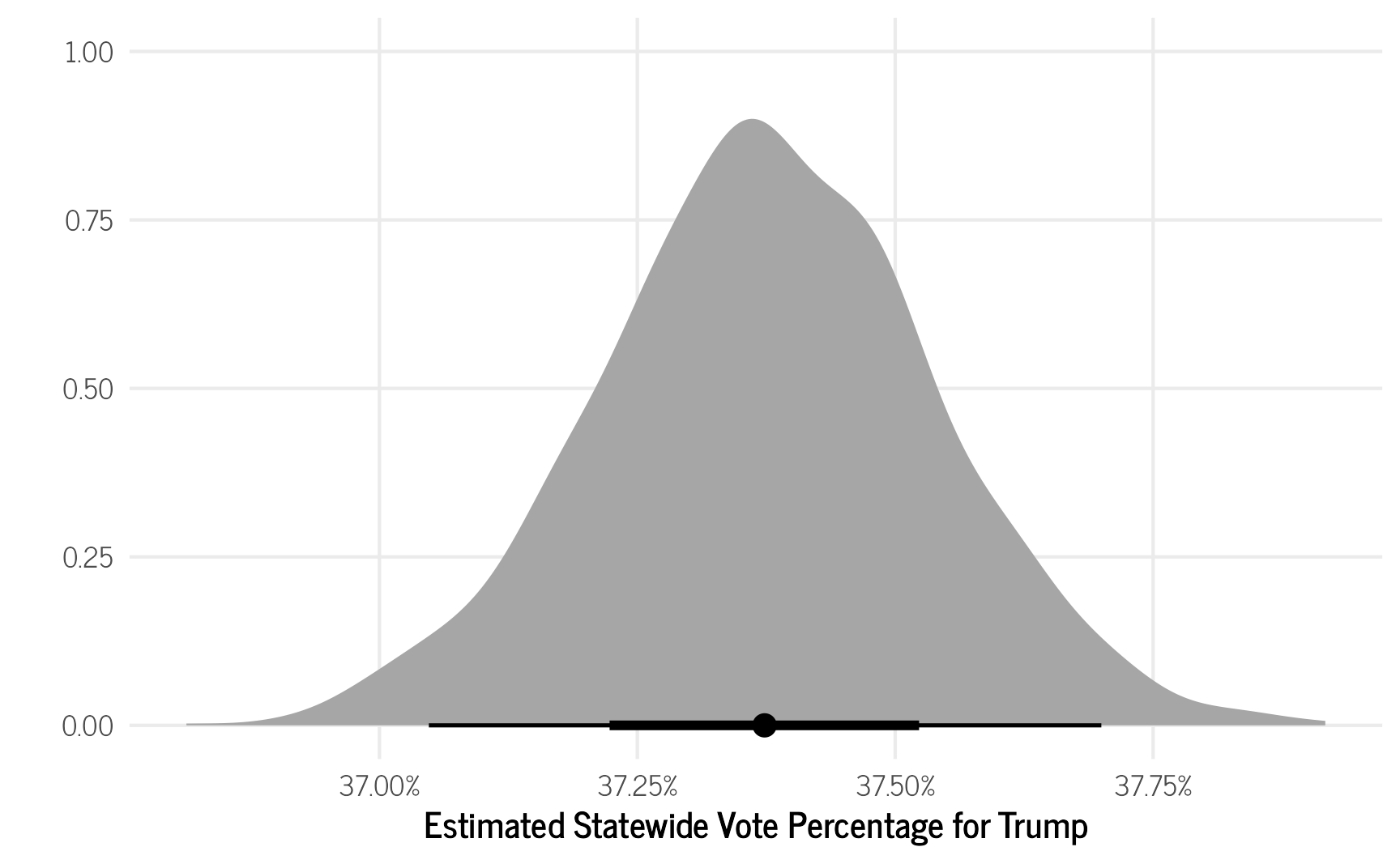
This new model still predicts that 37.37% of voters statewide supported Trump, which is the same as the observed percentage of 37.37% (excluding the three precincts that were removed for not having any neighbors).
Wrapping Up
Modelling the election results for Trump in Hawaiʻi using CAR models helped provide us with a better understanding of the level of support for Trump across the electorate in each of the state’s election precincts. Adding in census data to the model provided slightly more precise measures, but doesn’t substantially change the results. Finding a way to calculate the ACS’s measurement error for the aggregated results so that we could add that to the model may be helpful, as well as further examining which ACS variables to include. It may also be interesting to model the results based on the number of registered votes instead of the number of voters who actually voted. But I’ve already spent enough time thinking about Trump for now.
Futher Reading
For additional reading on CAR and other spatial models see:
Citation
BibTeX citation:
@online{rentz2025,
author = {Rentz, Bradley},
title = {Analyzing the {Results} of the 2024 {Presidential} {Election}
in {Hawaiʻi} {Using} {Bayesian} {Conditional} {Autoregressive}
{(CAR)} {Models}},
date = {2025-03-21},
url = {https://bradleyrentz.com/blog/2025/03/21/pres_election_hi_2024/},
langid = {en}
}
For attribution, please cite this work as:
Rentz, B. (2025, March 21). Analyzing the Results of the 2024
Presidential Election in Hawaiʻi Using Bayesian Conditional
Autoregressive (CAR) Models. https://bradleyrentz.com/blog/2025/03/21/pres_election_hi_2024/